Infer Statistical Package

Statistical inference deals with making some form of inference about the population under study based on a sample. The infer package provides a smooth workflow for conducting various inference tasks. Read on…

Author

Affiliation

Joash Geteregechi

Ithaca College department of mathematics. Views expressed here are my own, and do not represent the college’s position.

Introduction

Statistics is the bedrock of modern data analysis, enabling researchers and data scientists to draw meaningful conclusions from data. One crucial aspect of statistical analysis is statistical inference, which allows us to make predictions, test hypotheses, and estimate population parameters based on sample data. In the world of R programming, the infer package in RStudio is a powerful tool that simplifies and streamlines the process of conducting statistical inference. In this blog post, we’ll explore the infer package and learn how it can be harnessed to uncover hidden truths in your data.

What is the infer package?

The infer package is an R package that provides a user-friendly interface for conducting statistical inference. Developed by Hadley Wickham and other contributors, this package extends the capabilities of tidyverse by offering functions designed to perform essential inferential tasks. Whether you need to estimate confidence intervals, perform hypothesis testing, or compare groups, the infer package has got you covered.

Key Features and Functionalities

Point Estimates and Confidence Intervals:

One of the fundamental tasks in statistical inference is estimating population parameters from a sample. With the infer package, generating point estimates and constructing confidence intervals is a breeze. By leveraging the %>% pipe operator and other tidyverse functions, you can easily summarize your data, compute the point estimates, and calculate confidence intervals.

Hypothesis Testing:

The infer package streamlines hypothesis testing in R. It allows you to compare groups or test against a known value, with a choice between parametric and non-parametric methods. Whether you are dealing with one-sample, two-sample, or paired data, the package offers intuitive functions to conduct t-tests, Wilcoxon tests, and much more.

Bootstrapping:

Bootstrapping is a powerful resampling technique for estimating the sampling distribution of a statistic. The infer package makes bootstrapping easy, enabling you to generate thousands of resamples, calculate confidence intervals, and visualize the results.

Regression Inference:

When dealing with regression models, the infer package enables you to assess the statistical significance of coefficients and compare models using the lm() or glm() functions. It also simplifies the process of generating predictions and confidence intervals for the response variable.

Randomization Tests:

Randomization tests, also known as permutation tests, are invaluable when you cannot make assumptions about the underlying data distribution. The infer package empowers you to perform randomization tests effortlessly, helping you draw valid conclusions from non-parametric data.

Examples of Statistical Inference with infer

You can use the package to perform theory-based or simulation-based inference. I will walk you through how to perform each one of these for a single mean. I will use a data frame called gss (general social survey).

Suppose we want to use our sample data to test the hypothesis that the population mean time (in hours) is different from 40 (this test is two-sided). Here are the hypotheses in words and in symbols:

• Null hypothesis: \(H_0:\mu=40\), the population means is 40 hours.

• Alternative hypothesis: \(H_a: \mu \neq 40\), the population mean is not 40 hours.

Simulation-based inference

1. Calculate the observed statistic (i.e., sample mean for hours variable), saving it as x_bar.

   x_bar <- gss %>%
   specify(response = hours) %>%
   calculate(stat = "mean")

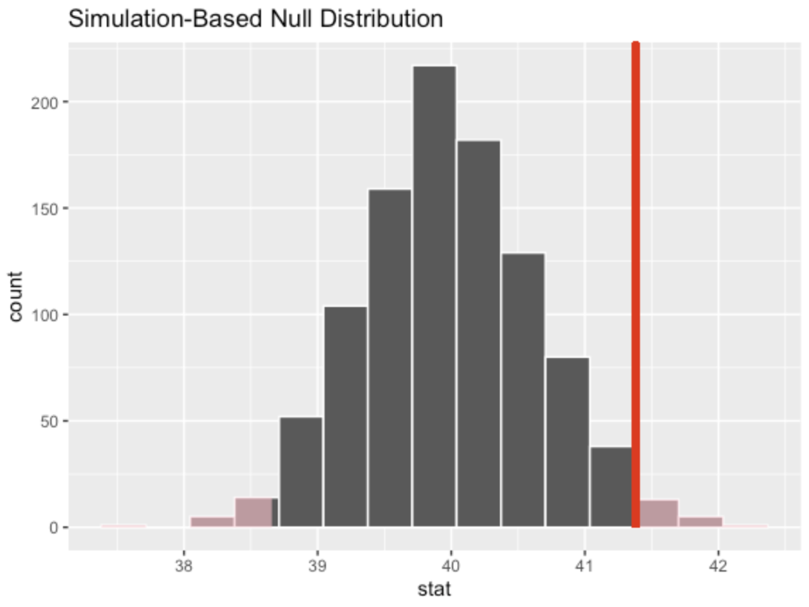
2. Create the simulation-based null distribution. Here, we are simulating 1000 statistics (means) which we can then graph (next step) to visualize their distribution:

   null_dist <- gss %>%
   specify(response = hours) %>%
   hypothesize(null = "point", mu = 40) %>%
   generate(reps = 1000) %>%
     calculate(stat = "mean")

3. (Optional step) Visualize the (sampling) distribution:

   visualize(null_dist) +
   shade_p_value(obs_stat = x_bar, direction = "two-sided")

   

   .

4. Calculate the p-value and write your conclusion:

   null_dist %>%
   get_p_value(obs_stat = x_bar, direction = "two-sided")

Theory-based (t-test) inference

The theory-based inference assumes the t-distribution (must check all conditions) to find the p-value. Below are the steps:

1. Calculate the observed statistic (the T-score) and save it as t_bar:

   t_bar <- gss %>%
   specify(response = hours) %>%
   hypothesize(null = "point", mu = 40) %>%
   calculate(stat = "t")

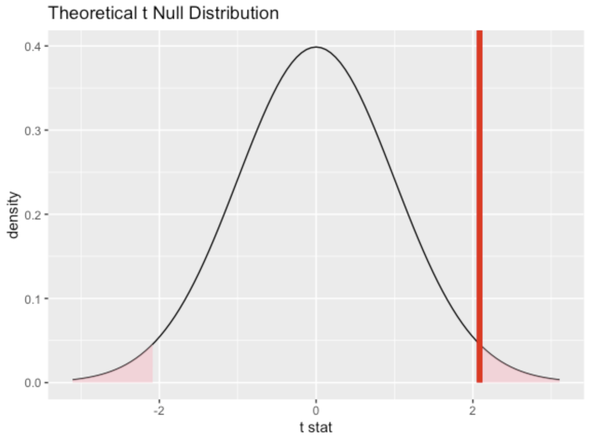
2. Generate the null distribution assuming the t-distribution:

   null_dist_theory <- gss %>%
   specify(response = hours)  %>%
   assume("t")

3. Visualize

   visualize(null_dist_theory) +
   shade_p_value(obs_stat = t_bar, direction = "two-sided")

.

4. Compute the p-value for your test and write the conclusion:

   null_dist %>%
   get_p_value(obs_stat = t_bar, direction = "two-sided")

To learn more about how to use infer for inference on other statistics, visit the infer website. The website also provides ways to create confidence intervals, which are are a very important part of statistical inference.