Lab 03a

Introduction

In today’s lab, we introduce an interface known as quarto that is helpful in creating reproducible reports. You will recall that in our first two labs, we used R scripts and had to copy and paste stuff from R into a word document for submission. With a quarto file, we don’t have to do this. You can generate (render) documents in different formats (e.g., pdf, word, etc) for sharing and submission. Quarto allows you to write both code and plain text in the same document. The code has to be written in what is known as code chunks while the non code text goes to the white spaces of the page. Recall that in an R script, we had to use comments for non code text. In general, while R scripts are great, they make it incredibly hard to reproduce and share your analyses with others. If you are using the desktop version of RStudio, you need to download quarto from https://quarto.org/docs/get-started/ before you proceed.

We will also learn to use the Tidyverse package (introduced and installed during lab 1) to perform basic summary statistics. Furthermore, we will introduce ggplot2, a popular package for data visualization in R. The ggplot2 package is included in the Tidyverse package so we do not need to install it separately.

Creating a Quarto File

To create your First Quarto file, follow the following steps:

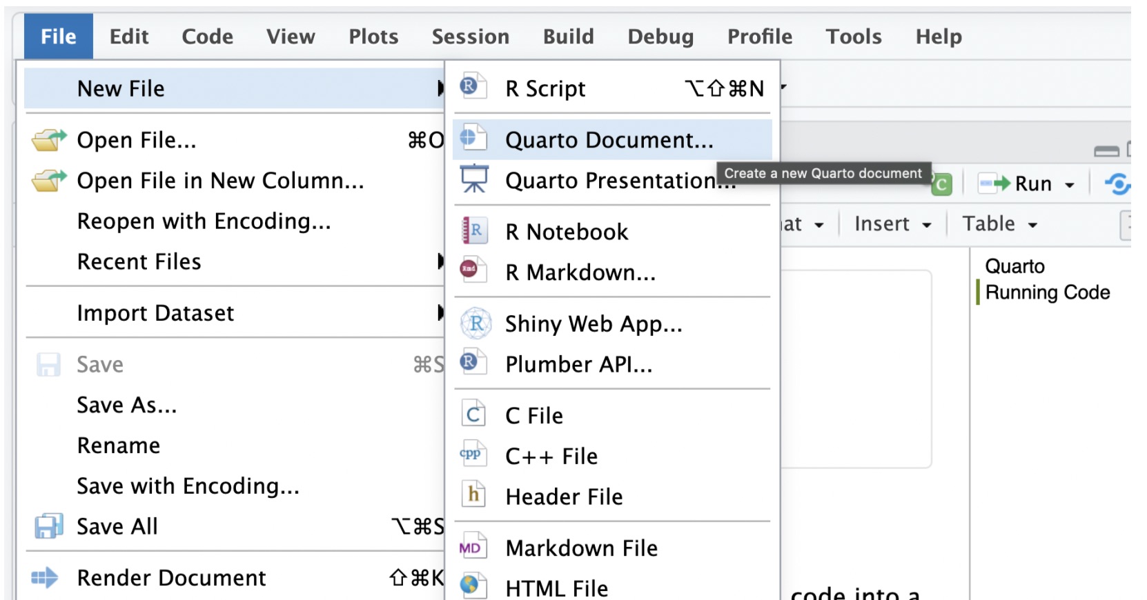
Go to File>New File > Quarto document. See below:

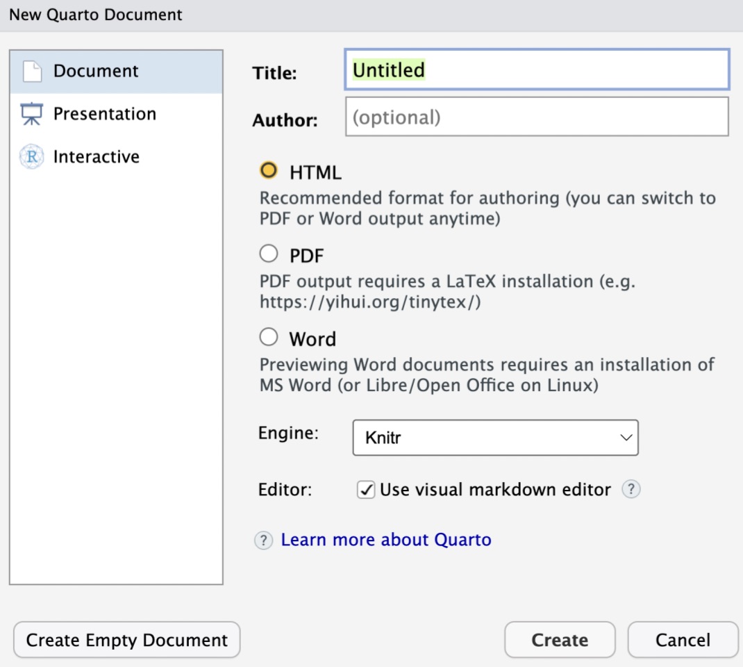
A pop up window will appear with fields for the title and author. Enter the title of the document as Intro to Quarto and Tidyverse. Under the author field, write your name. Change the output format to pdf. The popup window looks as follows:

Next, click on create. Note that the document appears with the name Untitled and is not saved yet to your files. To rename and save it, click on file then navigate to save then change the name from untitled to Lab_03a. The document should appear under the files section with a .qmd extension. With this document saved here, you can always return to it any time and continue working.

Rendering your Quarto File

To render means to process your quarto file and generating the output defined (in our case pdf). Rendering may not work if some of the code has errors. The good thing is that quarto will tell you where the errors occurred so you can fix them. If you want to see the exact line where the error occurred, you will need to use the source option instead visual. It is important to note that code will run line by line starting from the top. This means that your code must be ordered in some way. For example, if you need to use a function from a certain package (e.g., tidyverse), the package activation code (e.g., library(tidyverse)) has to run before using that function.

Creating Code Chunks in Quarto

You will note that the document we created already has both plain text and code chunks that come with the template. We can delete all the text and code chunk and create out own or edit what you have in the template. As indicated earlier, the code chunks are for writing code while the white spaces are for plain text. To add your own code chunk, just click on code then go to add new chunk or use the keyboard shortcut cmd+opt+I on a mac and control+opt+I on a Windows PC. When doing this, make sure your cursor is at the place where you want to create the new code chunk.

Note that Quarto supports other programming languages as well. If you want to write python code in quarto, you can create a python code chunk.

Using Code Chunks

In a code chunk, you write code that you want to reproduce in your report. There are other operations such as installing packages that should be done only in the console. Running the install.packages operation in a apckage will mean that quarto will try to install that package every time you render. Recall that we install packages only once. However, operations such as activating packages (i.e., library(package name)) may be included in the quarto file near the top of the document.

As a start, let us load the openintro, tidyverse, and palmerpenguins packages. Copy and paste the following code in the first code chunk:

library(openintro)
library(tidyverse)
library(palmerpenguins)

Run the code chunk to load the packages. If any of them is missing, R will prompt you to install them. In most cases, you do not need to include the code output for package activation in your report. To hide this output, you use #|include=false as shown below:

#|include=false
library(openintro)
library(tidyverse)
library(palmerpenguins)

Loading Data into quarto

We want to load a data set called duke_forest into our quarto file. Recall that the data set duke_forest is contained in the openintro package and so all we need to do it run the code data(duke_forest). Since data(duke_forest) is code, we need to put it in a code chunk. See below:

data(duke_forest)

We have already seen the data set duke_forest (see lab 2) but you can use the query command ?duke_forest to learn more about it.

Some Analyses (Using Tidyverse)

Summarizing Numerical variables

Let us start by finding various numerical summary statistics for the variable price in the duke_forest data set. To find the mean, create a code chunk and run the code shown below:

mean(duke_forest$price)

[1] 559898.7

The above is a base R code (does not draw from any package). We can achieve the same results by using the summarize function from the tidyverse package as shown below:

duke_forest|>
  summarize(mean(price))

# A tibble: 1 × 1
  `mean(price)`
          <dbl>
1       559899.

Here, the sign |> is called a pipe operator and we shall use it frequently. It sends anything on its left to its right. In this case, it sends the data into the summarize function. Inside the summarize function, you have to specify the summary statistic you want (in our case the mean).

Tidyverse uses the pipe operator a lot. Code written in this manner is (arguably) easier to read than the base R format. Not also that base R code can be quite cumbersome especially as you add more arguments.

Question:

• Compute the median, maximum(max), minimum(min), and the standard deviation (sd) for the price variable.

To compute the quartiles (first and third), you can use the following commands:

data("sinusitis")

duke_forest|>
  summarize(quantile(price, .25))

# A tibble: 1 × 1
  `quantile(price, 0.25)`
                    <dbl>
1                  450625

#Change .25 to .75 for the third quartile

Summarizing a categorical Variable

You can also summarize categorical variables using tables. Let us first imprt the data set sinusitis that we used during lab 2. The code for importing the data is as shown below:

data("sinusitis")

We can start by creating a simple table showing the distribution of cases according to self_reported_improvement (i.e., whether someone reported improvement or not):

sinusitis|>
  group_by(self_reported_improvement) |>
  tally() 

# A tibble: 2 × 2
  self_reported_improvement     n
  <fct>                     <int>
1 no                           35
2 yes                         131

When you run the code, we notice that an overwhelming majority (131) reported improvement.

The problem with the simple table above is that we do not see the distribution of improvement in each group. To do this, we can create a contingency table: Use the code below:

sinusitis|>
  group_by(group, self_reported_improvement) |> 
  tally() |>
  spread(key = group, value = n)

# A tibble: 2 × 3
  self_reported_improvement control treatment
  <fct>                       <int>     <int>
1 no                             16        19
2 yes                            65        66

We can now see that 65 of the cases that reported self improvement were in the control group while 61 were in the treatment group. Does this suggest the treatment was effective? Why?

Another thing you may notice is that we do not have the totals. To add these you can use the adorn_totals function found in the janitor package. The program may prompt you to install the janitor package. Go ahead and install it.

sinusitis |>
  group_by(group, self_reported_improvement) |>
  tally() |>
  spread(key = group, value = n) |>
  adorn_totals(where = "both")

 self_reported_improvement control treatment Total
                        no      16        19    35
                       yes      65        66   131
                     Total      81        85   166

Question:

• Based on the above, table, what percent of cases in the treatment group reported improvement? What percent in the control group reported improvement?

Exercises

There are no exercises for today.