Lab 01

Introduction

In today’s lab, we introduce an interface known as quarto that is helpful in creating reproducible reports. One of the most powerful features of quarto is the fact that you can write code (in code chunks) and plain text in the same document. You can generate (render) your work into formats such as pdf, word, html, etc that can be shared easily. If you are using the desktop version of quarto, you need to download it from https://quarto.org/docs/get-started/ before you proceed.

Installing a new package

We are going to need a package called palmerpenguins. Install it before you proceed. To install the package, run the following command in the console:

install.packages("palmerpenguins)

Creating a quarto file

To create your First Quarto file, follow the following steps:

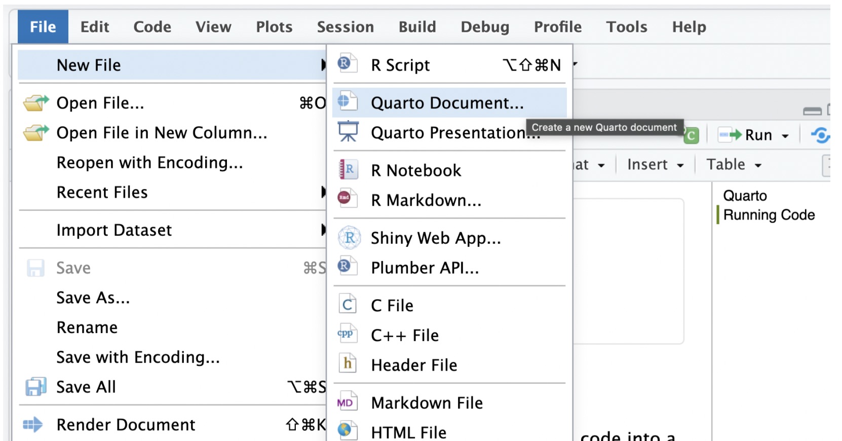
Go to File>New File > Quarto document. See below:

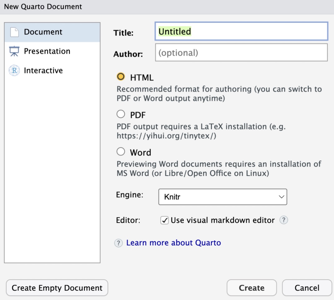
After clicking Quarto document,a pop up window will appear with fields for the title and author. Enter the title of the document as Introducing Quarto and Tidyverse because that is what we are doing today. Write your name under author. The output format can stay as HTML. You can always change these things even after creating the document. The popup window looks as follows:

Click create to create the document. Note that the document appears with the name Untitled. Click on file then navigate to save then change the name from untitled to Lab_01. Remember, we do not want to use a space for the document name. To tell whether your document saved properly, you will see the document under files with a .qmd extension. With this document saved here, you can always return to it any time and continue working.

Now, click on Render to see the output of the document you just created. You will note that the document has both plain text and code chunks. We shall use the code chunks for writing code and plain text for interpreting our analyses and writing reports. To add your own code chunk, just click on code the go to add new chunk or use the keyboard shortcut cmd+opt+I on a mac and control+opt+I on windows. When doing this, make sure your cursor is at the place where you want to create the new code chunk.

By default, the code chunk that comes is for R code. If you want to write python code, just change the r to python.

To create a new code chunk, you can copy an already existing code chunk and paste it elsewhere on the document then edit it appropriately. You may also create new code chunks by clicking on Code and navigating to Insert code chunk.

Using Code Chunks

In a code chunk, you write code that you want to reproduce in your report. There are other operations such as installing packages that should be done only in the console. When you render a quarto document, quarto runs all code chunks sequentially from top to bottom in order to output your report (in pdf, html, or word). If any code chunks has code for package installation, it means R will try to re-install the package every time you render the document (we said packages are installed one). Operations such as activating packages, i.e., library(package name), should be included in the first code chunk.

As a start, let us load the openintro, tidyverse, and palmerpenguins packages. Copy and paste the following code in the first code chunk:

library(openintro)
library(tidyverse)
library(palmerpenguins)

Run the code chunk with the packages to ensure that they are all working. If any of them is missing, R will prompt you to install them.

Loading (and viewing) Data

Remember that the openintro package contains the data that comes with the openintro text. To view a complete list of the data frames, visit https://www.openintro.org/data/. Today, we will use a data frame called penguins contained in the palmerpenguins package. To learn more about this data frame, run the following code in the console:

?penguins

To load the data into your document, run the following command:

data("penguins")

When you run the above code, a new object should appear in the environment area. Click on penguins to view and study the data.

Some Analyses (with Tidyverse)

Now that you have “imported” the data into R, we want to perform a few analyses. We are going to use the tidyverse package to do this. The tidyverse is a collection of R packages for data analysis that are developed with common ideas and norms. According to @Wickham2019,

“At a high level, the tidyverse is a language for solving data science challenges with R code. Its primary goal is to facilitate a conversation between a human and a computer about data. Less abstractly, the tidyverse is a collection of R packages that share a high-level design philosophy and low-level grammar and data structures, so that learning one package makes it easier to learn the next.”

Tidyverse Workflow

In lab_00, we performed the analyses using base R code. We saw that to compute the mean of a given variable in a data frame, you use data_frame_name$variable_name. The tidyverse workflow is a bit different and is what we shall use for the most part.

For example, to compute the mean of bill_length_mm from the penguins data frame, base R code would be

mean(penguins$bill_length_mm)

Try the code to see if it works. If not, what is the problem and how would you fix it?

In the tidyverse, the code for the mean of the bill length would be

penguins %>% summarize(length_mean = mean(bill_length_mm))

The symbol %>% is called a pipe and is very common in tidyverse. It takes anything on its left and sends it (pipes it) to the function on the right. Here, we are taking the mtcars data frame and piping it into the summarize function (the function for summary statistics). Inside the function, we specify the variable and the statistic (in this case the mean). We have chosen to name the result as length_mean but this could be changed.

You can compute other summary statistics in a similar manner as above and if there is an NA one way to deal with would be to remove it. In some cases, one would replace NA with the average of the other values.

Visualizing with ggplot2

In this section, we will start by creating scatter plots and then proceed to bar plots. You will learn about more visualization tools in later labs.

Scatter plots

Suppose we want to answer the following question: Do penguins with longer flippers weigh more or less than penguins with shorter flippers?

We will use a package called ggplot2 (part of tidyverse) to create a scatter plot to visualize the association between flipper length and and body weight.

ggplot2 is a package (part of the tidyverse umbrella) that is used to create nice-looking graphics. It adopts the grammar of graphics, which is a coherent system for describing and building graphs.

You provide the data, tell ggplot2 how to map variables to aesthetics, what graphical primitives to use, and it takes care of the details.

With ggplot2, you begin a plot with the function ggplot(), defining a plot object that you then add layers to sequentially until you get the desired plot. We will do this in steps:

• Step 1: Add the data:

  ggplot(data = penguins)

This creates an empty canvas

• Step 2: Provide the information about the x-axis and the y-axis (i.e., what variable do you want where?). We call this a mapping.

ggplot(
  data = penguins,
  mapping = aes(x = flipper_length_mm, y = body_mass_g)
)  

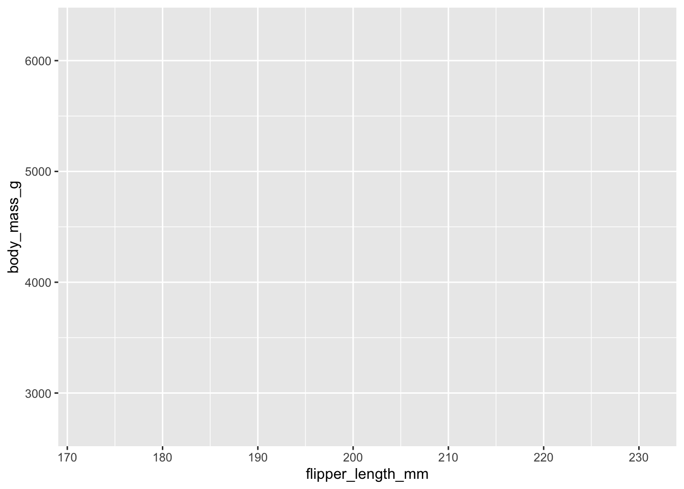
The above code adds to our empty canvas the variables specified for the y axis and the x-axis. We still do not have a scatter plot.

• Step 3: Define the geometry (geom) that you want ggplot2 to use. In our case, we want to use points and so we use the function geom_point(). Notice that you must have the parentheses because this is a function that can take arguments (you will learn more about this). Use teh code below:

ggplot(
  data = penguins,
  mapping = aes(x = flipper_length_mm, y = body_mass_g)
) +
  geom_point()

Warning: Removed 2 rows containing missing values (`geom_point()`).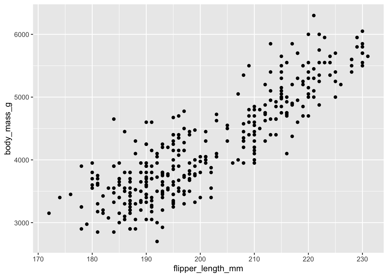

We finally have our scatter plot. Based on this scatter plot, what can you say about the question we sought to answer?

Remember the steps:

• Give ggplot the data,
• provide a mapping, and
• define a geometry using geom_.

Question: Try to change the geometry above to a histogram, i.e.,

ggplot(
  data = penguins,
  mapping = aes(x = flipper_length_mm, y = body_mass_g)
) +
  geom_histogram()

Does it work? If not, why?

Adding more aesthetics

The scatter plot above is a great tool to visualize the relationship between the two variables (flipper length and weight). Suppose we want to add a third (categorical) variable such as species to the scatter plot. We can achieve this by adding a third argument such as color to the aesthetics). See code below:

ggplot(
  data = penguins,
  mapping = aes(x = flipper_length_mm, y = body_mass_g, color=species )
) +
  geom_point()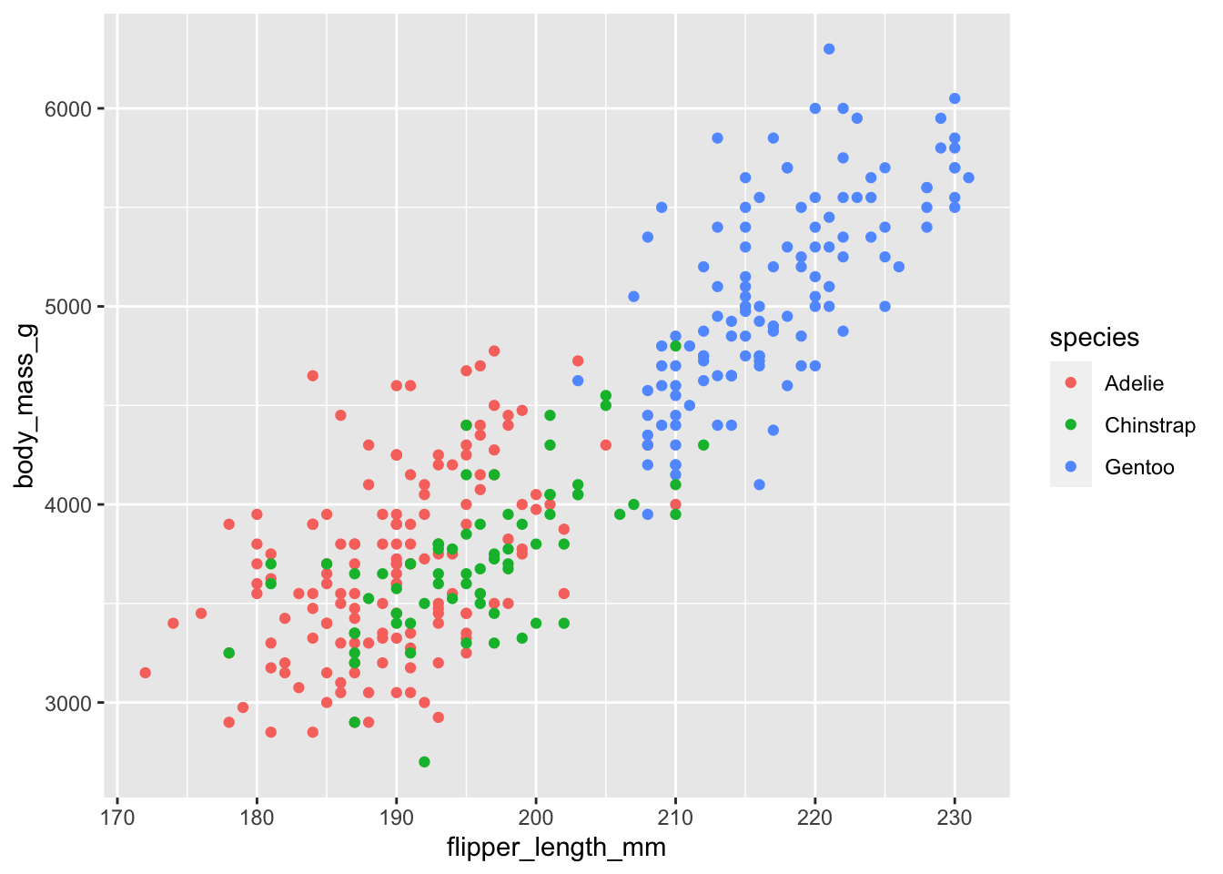

What do you learn from this new scatter plot that you do not from the first?

You can also visualize how the different species are scattered on the same scale by using the face_wrap function. See code below

ggplot(
  data = penguins,
  mapping = aes(x = flipper_length_mm, y = body_mass_g)
) +
  geom_point()+
  facet_wrap(~species)

Warning: Removed 2 rows containing missing values (`geom_point()`).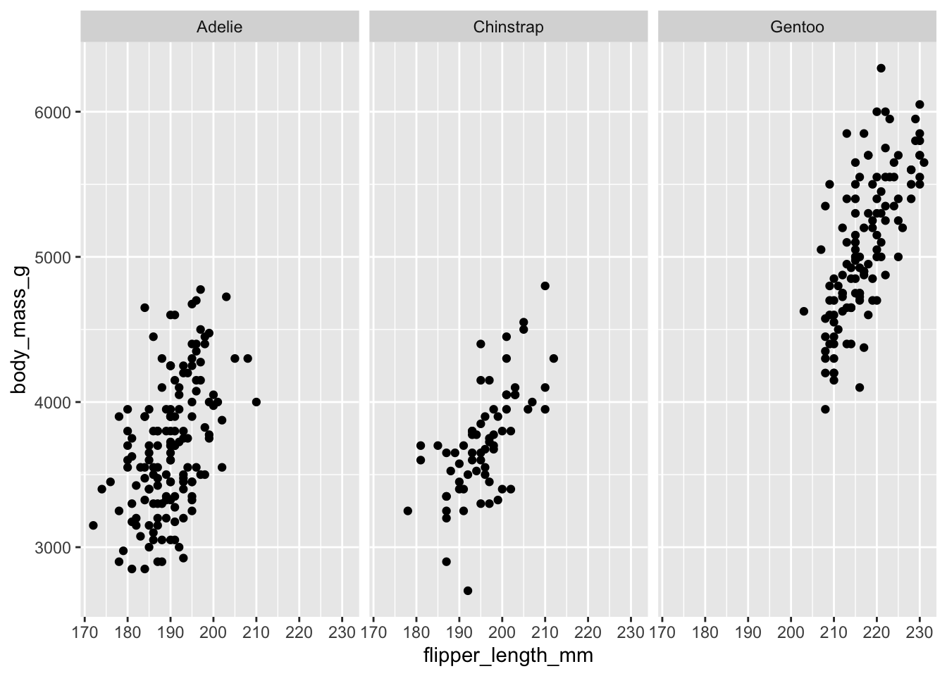

You can also add a numerical variable such as bill_depth_mm. See code below:

ggplot(
  data = penguins,
  mapping = aes(x = flipper_length_mm, y = body_mass_g, color=bill_depth_mm )
) +
  geom_point()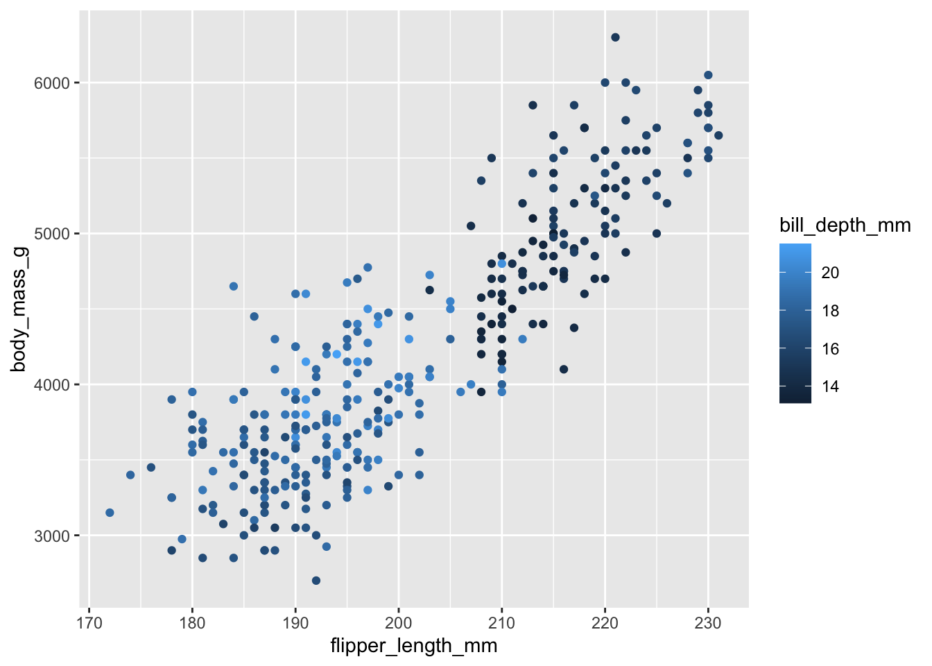

What do you learn from this scatter plot that you do not from the first?

Creating bar plots

You can also create bar plots in a similar manner as above. Remember that bar plots are for categorical variables. For example, we can use a bar plot to visualize the species of the penguins. See code below:

ggplot(penguins, aes(x = species)) +
  geom_bar()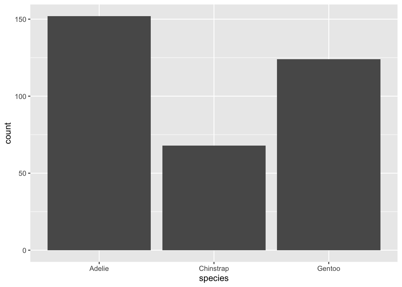

The above bar plot simply gives us the count for each species. If you wanted to color the bars by species, you can

ggplot(penguins, aes(x = species, color=species)) +
  geom_bar()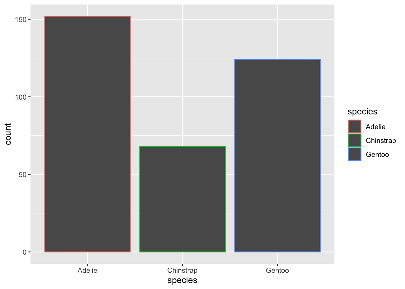

You can make the colors to fill the bars by using fill instead of color. See below:

ggplot(penguins, aes(x = species, fill=species)) +
  geom_bar()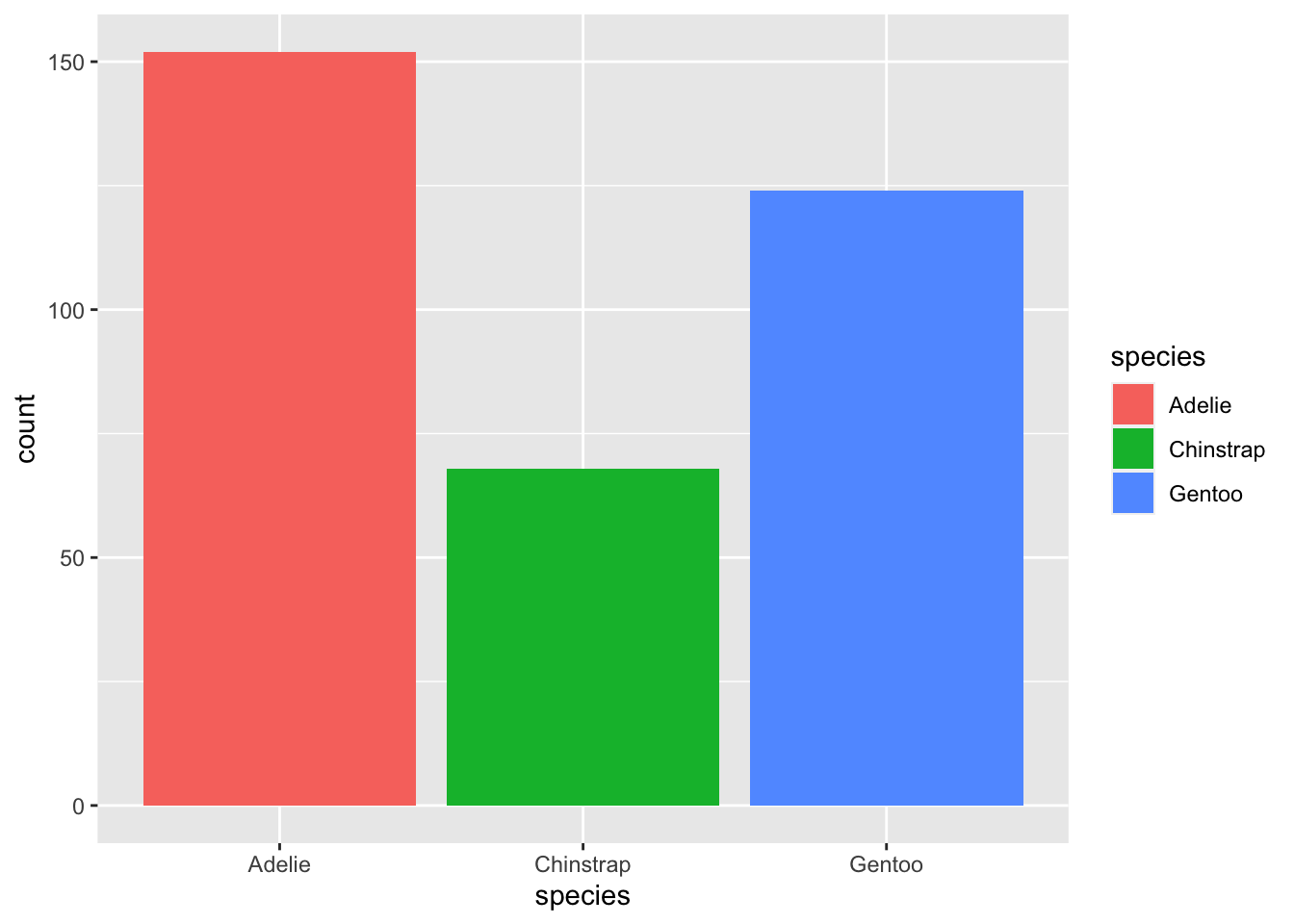

If you wanted to add another categorical variable such as island to visualize the relationship, you can fill by island nstead of by species. See below:

ggplot(penguins, aes(x = species, fill = island)) +
  geom_bar()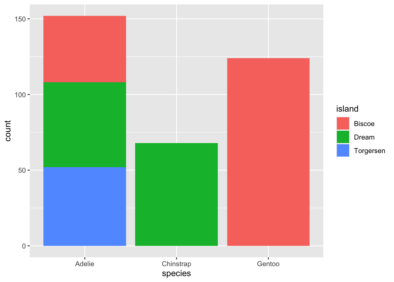

The problem with this bar plot is that it is difficult to interpret. We often prefer to have side-by-side bar plots. To achieve this, we add an argument called position inside the geom_bar function and set it to dodge.

ggplot(penguins, aes(x = species, fill = island)) +
  geom_bar(position = "dodge")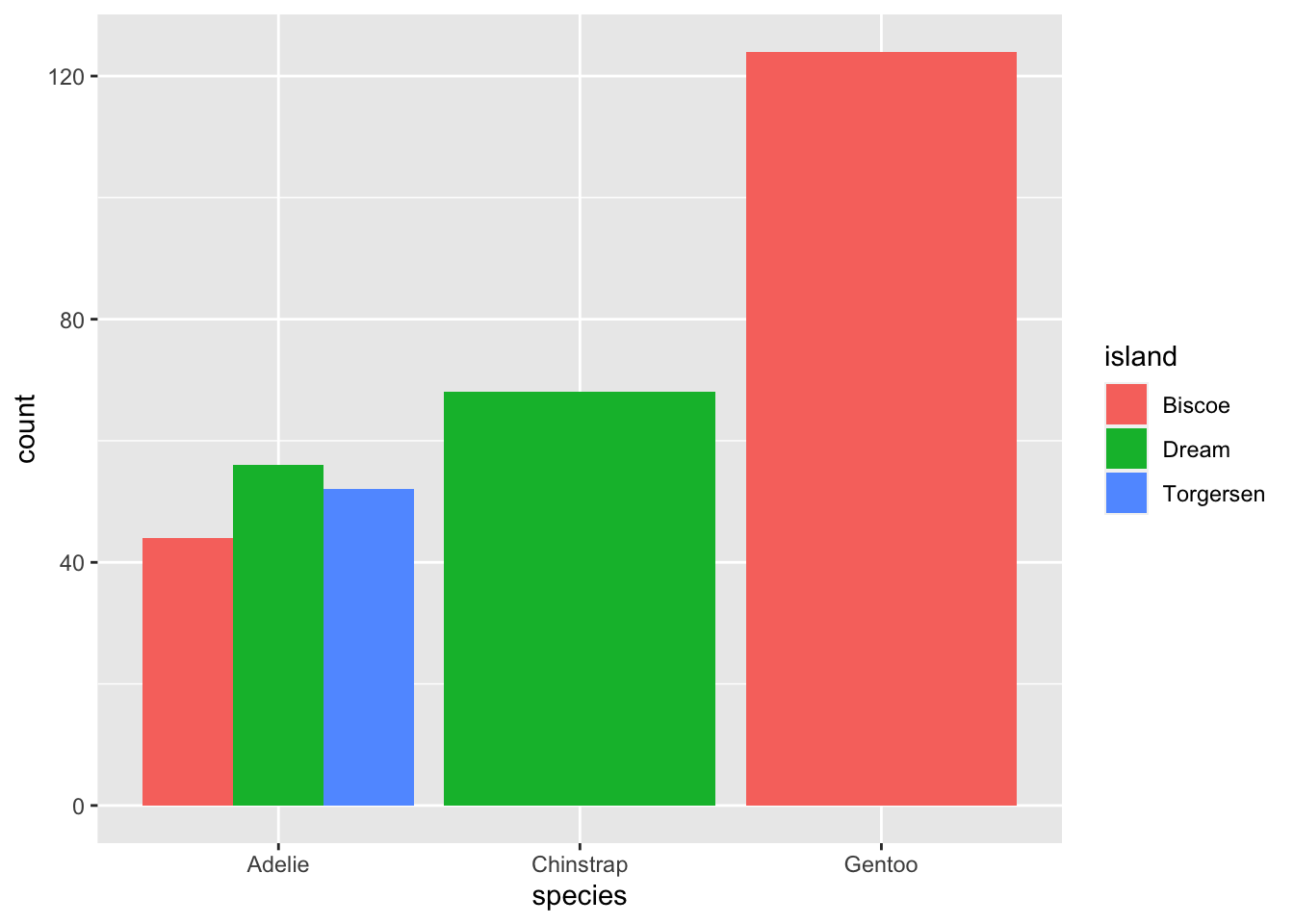

Exercises

1. (2 pts) There is a data frame called loan50 that is contained in the openintro package. load the data frame into your work space.
2. (2 pts) Give a brief description of this data frame. How many variables does the data frame have? How many cases/observations does it have?
3. (4 pts) Do people that have been employed for long tend to get lower interest rates? To answer this question, create a scatter plot for the variables emp_length and interest_rate.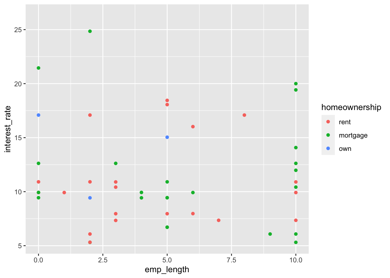
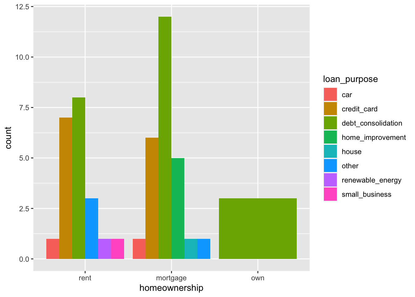
4. (4 pts) Recreate the following plot using the loan50 data frame.

5. (4 pts) Create a bar plot (with differently colored bars) to visualize the distribution of the loans by homeownership. What insights can you draw from this bar plot?

6. (4 pts) Recreate the following plot using the loan50 data frame.