Lab 06a

Introduction

In today’s lab activity, we will learn how to randomly sample from a given population and create a sampling distribution for proportion. Suppose you have a bag with a mix of 270 red and 330 white beans. This means that the proportion of red beans in the bag is, \(p= \frac{270}{600} = 0.45\). The goal is to take random samples from this population, create a sampling distribution, and examine its properties. You will also learn about the Central Limit Theorem (for proportion) in the process.

Creating your Quarto File

Sign in to posit cloud account and open the MATH 145 Class project. https://posit.cloud/
Clean up your work space then create a new Quarto file with the title Intro to inference.
Save the file as lab_06a. If you did everything correctly, a file named lab_06a.qmd should appear under the files section.

Loading Packages

Today, we will need the tidyverse and infer packages. Load these packages into your document. Use the code below:

library(tidyverse)
library(infer)

Run the code chunk to load the packages. If any of them is missing, R will prompt you to install them. Go ahead and install the package.

Modelling the population

We want to create a model for our population. We will use a character vector with the words Red and White. There will be 270 Red and 330 White to match our bag. See below:

Code

bean_color <- c(rep("Red", 270), rep("White", 330))

Next, we want to store this vector as something called a tibble (nice-to-work-with tables in R). To do this, we just pass the vector bean_color through the tibble function. See below:

Code

beans_bag <- tibble(bean_color)

Taking a random sample

Next, we sample 40 beans randomly from the bag (beans_bag) and save the sample as sample_1. The function that does random sampling from a defined population is called sample_n. See code below:

Code

sample_1<- beans_bag |>
                sample_n(40)

Compute proportions

Next, let us calculate the proportion of red beans in sample_1 create above. The code below starts by counting the beans by color and then computing the proportions for each color. We name the new column in the tibble as p-hat. See code below:

Code

sample_1 |>
              count(bean_color) |>
              mutate(p_hat = n /sum(n))

# A tibble: 2 × 3
  bean_color     n p_hat
  <chr>      <int> <dbl>
1 Red           19 0.475
2 White         21 0.525

You can repeat this process several times then collect all statistics (sample proportions). For each repeat you will need to rename the sample accordingly.

Multiple samples at once

At this point, it should be obvious that the above process can be tedious. There is a way to do it all at once using the rep_sample_n function from the infer package. In the code below, we are creating an object called sample_props40 which contains 10,000 random samples drawn from beans_bag with replacement. We are also filtering the data so we only have the proportion for red beans.

Code

sample_props40 <- beans_bag |> rep_sample_n(size = 40, reps = 10000,
                                replace = TRUE) |>
                                count(bean_color) |>
                                mutate(p_hat = n /sum(n)) |>
                                filter(bean_color == "Red")

Visualizing the Sampling Distribution

Finally, we can create a histogram to visualize the 10,000 sample proportions created above. Note that we stored the data set as an object called sample_prop40. Use code below:

Code

ggplot(data=sample_props40, aes(x=p_hat))+
              geom_histogram(binwidth = 0.01)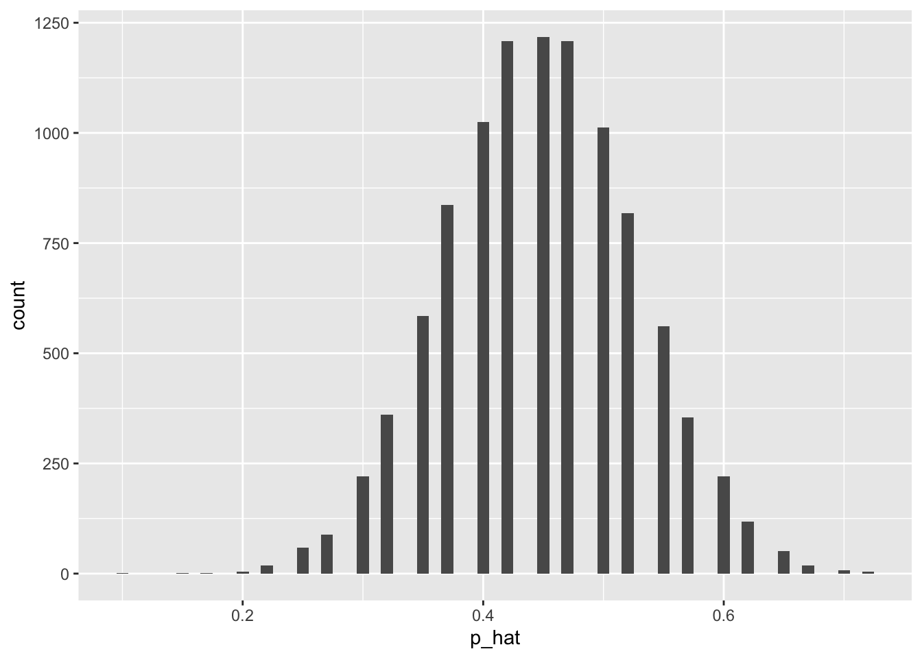

Summary Statistics for Sampling Distribution

We can compute the mean and the standard deviation of the sample proportions. See the base R code below:

Code

mean(sample_props40$p_hat)

[1] 0.449955

Code

sd(sample_props40$p_hat)

[1] 0.07901343

In Your Groups

Create a new sampling distribution with 10,000 samples each of size 80. Call this distribution sample_props80. Create a histogram to visualize the distribution (p_hat) and compute the mean and standard deviation.
Create a new sampling distribution with 10,000 samples each of size 100. Call this distribution sample_props100. Create a histogram to visualize the distribution (p_hat) and compute the mean and standard deviation.
What patterns do you notice? Specifically, talk about the mean, the standard deviation, and the features of the histogram.

“As you increase the sample size,….”