In today’s lab, we will run a hypothesis test for difference in two proportions using a function called prop.test, then proceed to use simulation-based approach. The prop.test function is used when the CLT conditions are met while the simulation-based approach can be used even when the sample proportion does not follow a normal distribution. Note however that independence is still necessary.
Creating your Quarto File
Sign in to posit cloud account and open the MATH 145 Class project. https://posit.cloud/
Clean up your work space then create a new Quarto file with the title Inference for Difference in two Proportions.
Save the file as lab_07. If you did everything correctly, a file named lab_07.qmd should appear under the files section.
Loading Packages
We will need the tidyverse and infer packages. Load these packages into your document. Use the code below:
library(tidyverse)library(infer)
Run the code chunk above to load the packages. If any of them is missing, R will prompt you to install them. Go ahead and install the package.
Scenario Description
Stents are devices put inside blood vessels that assist in patient recovery after cardiac events and reduce the risk of an additional heart attack or death. Many doctors have hoped that there would be similar benefits for patients at risk of stroke. A study was conducted to examine the effectiveness of stents in preventing strokes. The randomly sampled patients were randomly assigned to either the control or treatment group. Patients in the treatment group received stents but those in the control group did not. Each patient was monitored to check whether they had a stroke or not (no event) within the first 30 days and within 365 days of the program. The data below summarizes results for the first 30 days.
State the Hypotheses
Null Hypothesis(in words): Stents are not associated with higher rates of stroke among patients. The observed difference between the control and the treatment group was due to random chance.
Null Hypothesis(in symbols):\(H_0: p_1 - p_2=0\) Where \(p_1\) and \(p_2\) are the proportions of patients who have a stroke in the control and treatment group respectively.
Alt. Hypothesis(in words): There is something to the theory that infants are genuinely more likely to pick the helper toy (for some reason).
we also check for the second sample: \(n_2\hat{p}_2 \ge 10\Rightarrow\)\(227\times \frac{214}{227}=214>10\). Similarly, \(n_2(1-\hat{p}_2) \ge 10\)
CLT-based Inference with prop.test
Since the CLT conditions are met, we can use the prop.test function to run the hypothesis test and find the confidence interval.
The prop.test function takes the following arguments:
x = the total number of successes in each group.
n = the sample size for each group
alternative = defines how the p-value will be computed (direction).
conf.level: defines the confidence level.
For our case, we will use the two-sided alternative hypothesis and a 95% confidence level. By default, the null hypothesis is set to 0 (assumes there is no difference between the groups).See code below:
    2-sample test for equality of proportions with continuity correction

data:  c(191, 214) out of c(224, 227)
X-squared = 9.0233, df = 1, p-value = 0.002666
alternative hypothesis: two.sided
95 percent confidence interval:
 -0.14987619 -0.03022922
sample estimates:
   prop 1    prop 2
0.8526786 0.9427313
Interpreting the output:
Notice that the p-value is very small (0.002666) and less than 0.05. This means that we have string evidence against the claim that stents are not associated with strokes. It is likely that the stents are causing the strokes.
The confidence interval means that we are 95% confident that the true difference in proportion of no stroke occurrences between the patients that use stents and those that do not is between -0.14987619 and -0.03022922. This interval does not include 0 hence 0 is not a plausible value (rejected under hypothesis test).
Try This:
Before you proceed, try to change the number of successes to 33, and 13 (i.e., the patients that had strokes in Treatment and Control groups). Does doing this change the output? Explain.
Simulation-Based Inference (SBI)
Hypothesis Testing
We can run the above inference using simulation-based inference (SBI) and end up with the same conclusion. SBI is commonly used especially when the sample size is not large enough. Note however, that independence is still necessary.
Step 1: Create a model (data set)
We create a data set (a tibble) with two variables - group (Treatment or control) and stroke (stroke or no_stroke). We will specify the numbers to match what we have in the scenario. See code below:
Note that when we have actual, we would not need to create a model. We would just use the actual data but specify variables accordingly.
You may want to create a contingency table to see the data. Use the code below:
Code
table(stents_data$group, stents_data$stroke)
            no_stroke stroke
  Control         214     13
  Treatment       191     33
Step 2: Calcualte the observed statistic (aka point estimate
The observed statistic is the difference in proportions of no stroke occurrences between the two groups. We can calculate this by simply finding the difference in proportions. See code below:
\[\frac{191}{224}-\frac{214}{227}=-0.901\]
Step 3: Create the Sampling Distribution
To run the hypothesis test, we can use the infer package (a very popular package for performing inferential statistics). This is a shortcut way of doing SBI. We will use the specify function to specify the model, the hypothesize function to specify the null and alternative hypotheses, and the generate function to generate several samples by way of permuting (akin to sampling with replacement). We will then use the calculate function to calculate the relevant statistic for each sample, in this case difference in proportions. See code below:
Code
sampling_distribution <- stents_data |>specify(stroke ~ group, success ="no_stroke") |>hypothesize(null ="independence") |>generate(reps =1000, type ="permute") |>calculate(stat ="diff in props", order =c("Treatment", "Control"))
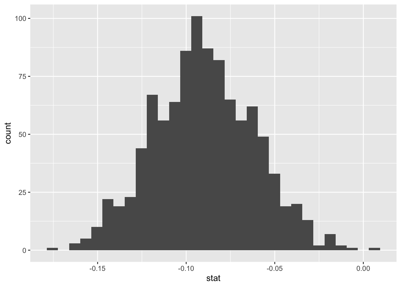
Step 4: Visualize the Sampling Distribution
You may want to visualize the sampling distribution. This is optional but it is good to confirm that the distribution is centered around the null value (in this case 0. See code below:
Finally, we can find the p-value by using the get_p_value function from the infer package. See code below:
Code
get_p_value(sampling_distribution, direction ="both", obs_stat =-0.0901)
Warning: Please be cautious in reporting a p-value of 0. This result is an
approximation based on the number of `reps` chosen in the `generate()` step.
See `?get_p_value()` for more information.
# A tibble: 1 × 1
  p_value
    <dbl>
1       0
Confidence Interval
Step 1: Create the Bootstrap Distribution
You start by creating the bootstrap distribution using the infer package. This is done by using the generate function with the type set to “bootstrap”. See code below:
Code
bootstrap_distribution <- stents_data |>specify(stroke ~ group, success ="no_stroke") |>generate(reps =1000, type ="bootstrap") |>calculate(stat ="diff in props", order =c("Treatment", "Control"))
Step 2: Visualize the Bootstrap Distribution Again, you may want to visualize the bootstrap distribution. This is optional but it is good to confirm that the distribution is centered around the observed statistic (aka point estimate). See code below:
Notice that with the interval and the P-value found by using SBI, we would reach the same conclusion as we did when using the prop.test function.
Exercises
Scenario Description:
In a study to determine the effectiveness of a new drug in treating a certain disease, 100 patients were randomly assigned to either the treatment group (50 patients) or the control group (50 patients). The results showed that 31 patients in the treatment group recovered while 12 patients in the control group recovered.
We may state the hypotheses for the above scenario as follows:
Null Hypothesis(in words): The new drug is not effective in treating the disease. The observed difference between the control and the treatment group was due to random chance. \[H_0: p_1 - p_2=0\]
Alternative Hypothesis(in words): There is evidence that the new drug is effective in treating the disease. \[H_a: p_1 - p_2 \neq 0\]
Run a hypothesis test to determine if there is evidence that the new drug is effective in treating the disease. Write your conclusion in context.
Find a 95% confidence interval for the difference in proportions of patients that recovered in the treatment and control groups. Write your interpretation/conclusion in context. State whether this interval is consistent with the hypothesis test result.