In today’s lab, we will run a hypothesis test for a single proportion using a function called prop.test, then proceed to use simulation-based approach. Notice that the prop.test function assumes that the sample proportion follows a normal distribution (according to the CLT) while the simulation-based approach can be used even when the sample proportion does not follow a normal distribution.
Creating your Quarto File
Sign in to posit cloud account and open the MATH 145 Class project. https://posit.cloud/
Clean up your work space then create a new Quarto file with the title Inference for Single proportion.
Save the file as lab_06b. If you did everything correctly, a file named lab_06b.qmd should appear under the files section.
Loading Packages
Today, we will need the tidyverse and infer packages. Load these packages into your document. Use the code below:
library(tidyverse)library(infer)
Run the code chunk above to load the packages. If any of them is missing, R will prompt you to install them. Go ahead and install the package.
Scenario Description
In a study reported in the November 2007 issue of Nature, researchers investigated whether infants take into account an individual’s actions towards others in evaluating that individual as appealing or aversive, perhaps laying for the foundation for social interaction (Hamlin, Wynn, and Bloom, 2007). In other words, do children who aren’t even yet talking still form impressions as to someone’s friendliness based on their actions? In one component of the study, 10-month-old infants were shown a “climber” character (a piece of wood with “googly” eyes glued onto it) that could not make it up a hill in two tries. Then the infants were shown two scenarios for the climber’s next try, one where the climber was pushed to the top of the hill by another character (the “helper” toy) and one where the climber was pushed back down the hill by another character (the “hinderer” toy). The infant was alternately shown these two scenarios several times. Then the child was presented with both pieces of wood (the helper and the hinderer characters) and asked to pick one to play with.
One important design consideration to keep in mind is that in order to equalize potential influencing factors such as shape, color, and position, the researchers varied the colors and shapes of the wooden characters and even on which side the toys were presented to the infants. The researchers found that 28 of the 32 infants chose the helper over the hinderer.
(NOTE: The study sample is slightly modified to fit our situation but the underlying statistics stay the same)
State the Hypotheses
Null Hypothesis(in words): Infants choose randomly and we happened to get “lucky” and find most infants picking the helper toy in our study.
Null Hypothesis(in symbols):\(H_0: p=0.5\)
Alt. Hypothesis(in words): There is something to the theory that infants are genuinely more likely to pick the helper toy (for some reason).
Alt. Hypothesis(in symbols):\(H_a: p>0.5\)
Checking CLT
The prop.test function assumes that the Central Limit Theorem (CLT) is satisfied. So, we have to check this first:
Independence: The observations/cases are independent because the sample was a random sample.
Sample size: The success condition: \(np \ge 10:\)\(32\times.5=16>10\). Similarly, \(n(1-p) \ge 10:\)\(32\times.5=16>10\). Thus, the sample is large enough for the CLT to apply.
Using prop.test function
The prop.test function takes the following arguments:
x = the total number of successes (i.e., how many cases meet the criteria under consideration, e.g., how many beans are red)
n = the sample size
p = the NULL value (value in the null hyp)
alternative = defines how the p-value will be computed (direction).
conf.level: defines the confidence level.
Se example below:
Code
prop.test(x=28, n=32, p =0.5,alternative =c("greater"),conf.level =0.95)
    1-sample proportions test with continuity correction

data:  28 out of 32, null probability 0.5
X-squared = 16.531, df = 1, p-value = 2.393e-05
alternative hypothesis: true p is greater than 0.5
95 percent confidence interval:
 0.7303346 1.0000000
sample estimates:
    p
0.875
Interpreting the output:
Notice that the point estimate (p-hat) is 0.875 and that the p-value is extremely small (0.00002393). This provides strong evidence against the null hypotheses meaning that the the behavior of the toys influence infants choices of an object to play with.
The confidence interval runs from 0.73 to 1.0 meaning that we are 95% confident that the true proportion of infants that choose the helper toy is between 0.73 and 1.0. This interval does not contain the null hence hence supporting out assertion that the null value (0.5) is not a plausible value.
Simulation-Based Inference (SBI)
We can run the above inference using simulation-based inference (SBI). One advantage of the SBI is that they work even when the sample size is not large enough. Note however, that independence is still necessary.
Step 1: Create a model
We create a model to represent the null hypothesis. We can use a set of cards with Blue and Green cards. Let us say that the Blue cards represents Helper while Green represents Hinderer. In this set, we need 50% Green and 50% blue (see null hypothesis).
Code
card_color <-c(rep("Blue", 50), rep("Green", 50))
Let us store the vector as a tibble:
Code
card_set<-tibble(card_color)
Multiple samples at once
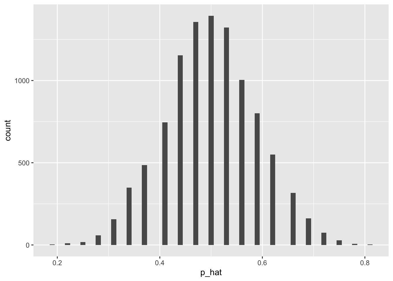
Let us use the rep_sample_n to take 10,000 random samples each of size 32. For each sample, we also calculate the proportion of blue cards. We will store the data as card_sample32.
Finally, we can create a histogram to visualize the 10,000 sample proportions created above. Note that we stored the data set as an object called card_sample32. Use code below:
Notice that the above data set has 0 cases. Thus, the P-value will be \(p-value=\frac{0}{10000}=0\).
Notice that this does not change teh conclusion made earlier.
SBI Confidence Interval
Recall that the CI is centered around the point estimate, not the null value]. This means we cannot rely on the simulation data created above. Instead, we will take our repeated samples from the sample in a process called bootstrapping.
See below:
Start by creating the sample model in R. We can call this vector choice.
Code
choice <-c(rep("Blue", 28), rep("Green", 4))
Convert choice into a tibble as shown below:
Code
sample_data<-tibble(choice)
Next, take repeated samples from this sample_data usinfg the rep_sample_n function. See below:
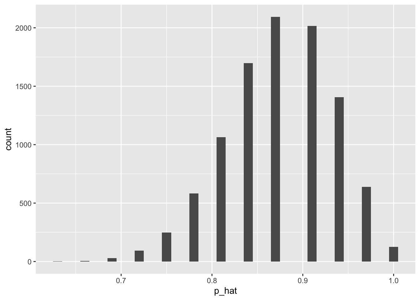
Next, we can graph this to visualize the bootstrap distribution. This is an optional step but it is good to confirm that your bootstrap sample is centered around the point estimate.
We notice that the distribution is centered around the point estimate (0.875) but has a slight left skewness. To find the confidence interval, we find the value that cuts off the bottom 2.5%. See the code below:
Code
quantile(bootstrap_samples$p_hat, probs =0.025)
2.5%
0.75
Next, we find the value that separates the top 2.5% from the bottom 97.5%. See below:
Code
quantile(bootstrap_samples$p_hat, probs =0.975)
  97.5%
0.96875
Thus, the 95% confidence interval is \((0.75,0.969)\)
Most people are right-handed and even the right eye is dominant for most people. Researchers have long believed that late-stage human embryos tend to turn their heads to the right. German bio- psychologist Onur Güntürkün (Nature, 2003) conjectured that this tendency to turn to the right manifests itself in other ways as well, so he studied kissing couples to see if both people tended to lean to their right more often than to their left (and if so, how strong the tendency is). He and his researchers observed couples from age 13 to 70 in public places such as airports, train stations, beaches, and parks in the United States, Germany, and Turkey. They were careful not to include couples who were holding objects such as luggage that might have affected which direction they turned. We will assume these couples are representative of the overall decision making process when kissing. In total, 124 kissing pairs were observed with 80 couples leaning right (Nature, 2003).
State the null and alternative hypotheses (in words and in symbols) for the above scenario.
Calculate the appropriate point estimate and determine whether its distribution would be normal or not. Show all work.
If the distribution is normal, what would be the mean and the standard deviation (standard error)?
Would you consider the point estimate found in #2 above unusual? Explain?
Determine the p-value for this scenario. What does this value tell you?
Summarize the conclusions you would draw from this study.
Create a 95% confidence interval and interpret it. Does this interval agree with the results of the hypothesis test? How so?