Code
data(heart_transplant)In the previous labs, we built models with numerical response variables only. In this lab, you will learn how to build regression models with a categorical (binary) response variable. This type of regression is called logistic regression and is one of the many generalized linear models (GLMs) that exist.
A well-known Stanford University study on heart transplants tracked the five-year survival rate of patients with dire heart ailments. The purpose of the study was to assess the efficacy of heart transplants, but for right now we will simply focus on modeling the survival rates of these patients. This plot illustrates how those patients who were older when the study began were more likely to be dead when the study ended (five years later).
Create a new quarto file with the title Intro to Logistic Regression and save the file as lab_4. If you are unsure how to do this, please refer to previous labs.
Please load openintro, tidyverse, statsr, GGally, broom, and Stat2Data Stat2Data is new so you will need to install it before you proceed. It has some data sets that you will need for the exercises section. To install the package, use the command:
install.packages("Stat2Data")Next, load the packages:
library(openintro)
library(tidyverse)
library(statsr)
library(broom)
library(GGally)
library(Stat2Data)
Run the packages before you proceed to make sure they loaded properly.
We will use a data frame called heart_transplant. It is contained in the openintro package so you can load it using the code:
data(heart_transplant)Before you proceed, please run the following command in the console to learn more about this data. If you don’t, the analyses and their interpretations won’t make sense to you.
?heart_transplantLet us start by creating a scatter plot to visualize the relationship between the variables age and survived (i.e., whether someone is still alive or not).
ggplot(data = heart_transplant, aes(x = age, y = survived)) +
  geom_jitter(width = 0, height = 0.02, alpha = 0.5)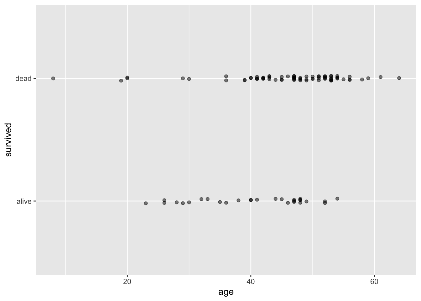
# We use a jitter to shake up the points a little bit
# Notice we have also added more arguments in the jitter.
# Try removing the extra arguments in the jitter to see what happens
First, we have a technical problem, in that the levels of our response variable are labels, and you can’t build a regression model to a variable that consists of words! We can get around this by creating a new variable that is binary (either 0 or 1), based on whether the patient survived to the end of the study. We call this new variable is_alive.
heart_transplant <- heart_transplant |>
  mutate(is_alive = ifelse(survived == "alive", 1, 0))
Below is a new scatterplot with a changed vertical axis. We are saving the object as data_space because we will need it later:
data_space <- ggplot(data = heart_transplant, aes(x = age, y = is_alive)) +
  geom_jitter(width = 0, height = 0.02, alpha = 0.5)
print(data_space)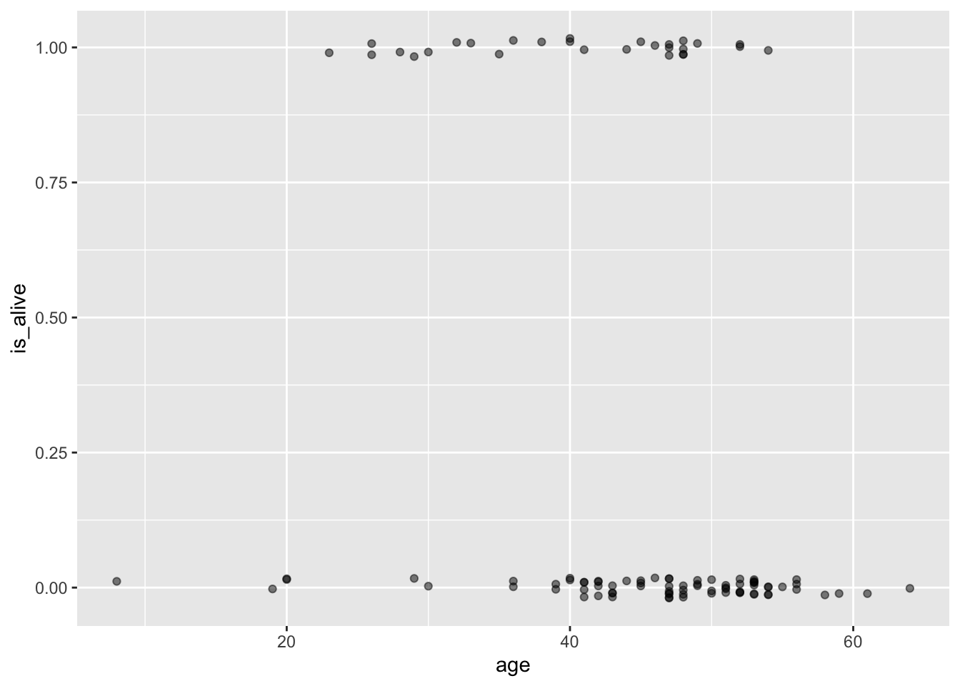
Now there is nothing preventing us from fitting a simple linear regression model to these data, and in fact, in certain cases this may be an appropriate thing to do.
But as we discussed in class, it’s not hard to see that the line doesn’t fit very well.
data_space +
  geom_smooth(method = "lm", se = FALSE, color="red")
`geom_smooth()` using formula = 'y ~ x'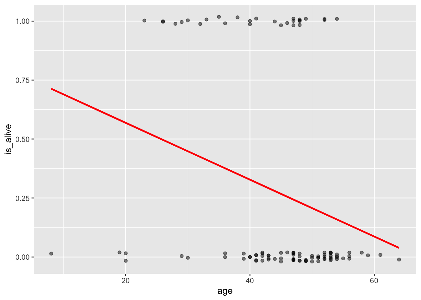
Limitations of regression of this model (linear)
What would this model predict as the probability of a 70-year-old patient being alive? It would be a number less than zero, which doesn’t make sense as a probability. Because the regression line always extends to infinity in either direction, it will make predictions that are not between 0 and 1, sometimes even for reasonable values of the explanatory variable.
Second, the variability in a binary response may violate a number of other assumptions that we make when we do inference in multiple regression. We will learn about those assumptions later when we cover inference for regression.
Thankfully, a modeling framework exists that generalizes regression to include response variables that are non-normally distributed. This family is called generalized linear models or GLMs for short. One member of the family of GLMs is called logistic regression, and this is the one that models a binary response variable.
A logistic regression model uses the logit function (discussed in class) to model relationships such as trhe one above:
\[ logit(p)=ln\left(\frac{p}{1-p}\right)= b_0+b_1x \]
The structure for fitting the logistic regression model is slightly different from the one used for linear regression. In the code below, we create the model (saving it as model_1) and then tidy it. Notice that we use the family argument to specify the type of glm that we want (in this case binomial because the response is binary).
model_1 <- glm(is_alive ~ age, family = binomial, data = heart_transplant)
tidy(model_1)
# A tibble: 2 × 5
term estimate std.error statistic p.value
<chr> <dbl> <dbl> <dbl> <dbl>
1 (Intercept) 1.56 1.02 1.54 0.123
2 age -0.0585 0.0231 -2.54 0.0112#NoticeWrite out the equation of the model and interpret the slope.
The raw model we created above models log odds, we can exponentiate the coefficients to get the odds. This makes it easier to interpret the model:
exp(coef(model_1))(Intercept) age
4.7797050 0.9432099 In the graph below, the blue line is the linear model (lm) while the red one is the logistic regression one (gml). Notice how the gml model is starting curve especially at the ends. The glm is asymptotic to 1 and 0 but the lm will cross these limits hence giving invalid results for certain values (e.g., predicting for someone who is 70). In this case, for most ages, the simple linear regression line and the logistic regression line don’t differ by very much, and you might not lose much by using the simpler regression model. But for older people, the logistic model should perform much better.
data_space +
  geom_smooth(method = "lm", se = FALSE) +
  geom_smooth(method = "glm", se = FALSE, color = "red",
              method.args = list(family = "binomial"))
`geom_smooth()` using formula = 'y ~ x'
`geom_smooth()` using formula = 'y ~ x'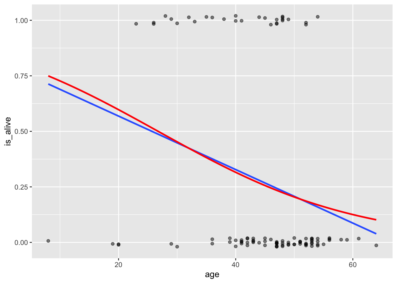
One important reason to build a model is to learn from the coefficients about the underlying random process. For example, in the Stanford heart transplant study, we were able to estimate the effect of age on the five-year survival rate. This simple model shed no light on the obvious purpose of the study, which was to determine whether those patients who received heart transplants were likely to live longer than the control group that received no transplant.
Let us create a new model by adding the variable transplant. We can call this new one model_2.
model_2 <- glm(is_alive ~ age + transplant,
                    data = heart_transplant, family = binomial)
tidy(model_2)
# A tibble: 3 × 5
term estimate std.error statistic p.value
<chr> <dbl> <dbl> <dbl> <dbl>
1 (Intercept) 0.973 1.08 0.904 0.366
2 age -0.0763 0.0255 -2.99 0.00277
3 transplanttreatment 1.82 0.668 2.73 0.00635Write the equation of the model and interpret the slopes for each predictor variable. Use your model to predict the status of someone who received a transplant and is 71 years old.
You can also exponentiate the coefficients as shown:
model_2 <- glm(is_alive ~ age + transplant,
                    data = heart_transplant, family = binomial)
exp(coef(model_2))
(Intercept) age transplanttreatment
2.6461676 0.9265153 6.1914009 There is a function called augment() that returns a data frame with—among other things — the fitted values (i.e., the log odds) for each observation. Let us run this function and store the data frame as aug_model_2:
aug_model_2<- augment(model_2)Take a look at aug_model_2. The variable/column .fitted are the log odds. It is more useful to get probabilities instead of log odds. To achieve this, you just add the argument type.predict to the augment() and set its value to response. Use code below:
aug_model_2_prob<- augment(model_2, type.predict = "response")If our response variable is binary, then why are we making probabilistic predictions? Shouldn’t we be able to make binary predictions? That is, instead of predicting the probability that a person survives for five years, shouldn’t we be able to predict definitively whether they will live or die?
There are a number of different ways in which we could reasonably convert our probabilistic fitted values into a binary decision. The simplest way would be to simply round the probabilities. We want to create a new data frame from the aug_model_2_prob that tells us (predicts) whether someone died or not in 5 years based on the predicted probability. Let us call this model model_2_plus.
model_2_plus <- aug_model_2_prob %>%
  mutate(alive_hat = round(.fitted))
#We round fitted to 0 or 1 and save it as a new column called alive_hatSo how well did our model perform? One common way of assessing performance of models for a categorical response is via a confusion matrix. This simply cross-tabulates the reality with what our model predicted. The code below tabulates the predicted outcomes (alive_hat) vs the actual ones (is_alive). we select the two variables of interest and then pipe them into the table() function as shown below:
model_2_plus %>%
  select(is_alive, alive_hat)%>%
  table()
alive_hat
is_alive 0 1
0 71 4
1 20 8In this case, our model predicted that 91 patients would die (see column with 0 for alive_hat), and only 12 would live (see column with 1). Of those 91, 71 actually did died, while of the 12, 8 actually lived. Thus, our overall accuracy was 79 out of 103, or about 77%.
In these exercises, you will use a data frame called MedGPA contained in the Stat2Data package.
(2 pts) Create a scatter plot to visualize the relationship between GPA (x-axis) and Acceptance (y-axis). Describe this relationship.
(2 pts) Create a new plot by adding a straight line (use lm method) to the plot in number 1 above.
(2 pts) Create a new plot by adding a curve (use glm method) to visualize the logistic regression model. Compare the plot in number 2 above to this new plot. Which one might better fit the data?
(2 pts) Create a logistic regression model for predicting Acceptance using GPA as the only predictor variable. Write down the equation of the model below and interpret its parameters (slope and intercept) in context.
(4 pts) Create a new logistic regression model by adding the variables Sex and MCAT to the model in number 4 above. Write down the equation of the model and interpret all slopes in context.
(4 pts) What does the model in number 5 above predict for the first case (first row) in the data frame MedGPA? Does the model make the correct prediction? What about the last case (row 55)?
(4 pts) Create a confusion matrix for the model in number 6 above. What is the accuracy (give as a percentage) of this model? Suggest some ways to improve the accuracy of the model.