Lab 06

Inference for Linear Regression (Single Predictor)

Introduction

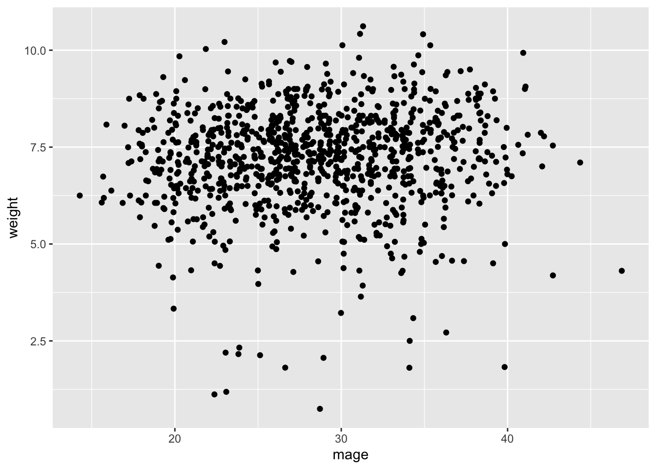
In this lab, we will perform statistical inference (hypothesis testing and parameter estimation using confidence intervals) for linear regression. We will start by examining a numerical predictor variable then proceed to a categorical predictor variable with two levels (equivalent to a t-test).

Numerical Predictor Variable

Prior studies have hinted at links between mothers’ age and child birth weight, as well as potential health consequences when babies are very small or very large. Babies who grow less than expected in the womb have a higher risk of birth complications, as well as diabetes and heart disease in adulthood. Very large newborns may be more likely to become obese later in life. For more details, see https://obgyn.onlinelibrary.wiley.com/doi/10.1111/j.1471-0528.2010.02823.x.

We want to answer the following research question via hypothesis testing:

Does a mother’s age influence a baby’s birth weight?

The Data

To answer the above research question, we will use a dataset called births14 contained in the openintro package.

Hypotheses

Null Hypothesis: There is no linear relationship between mothers’ age and birth weight.

In symbols: \(H_0:β=0.\)

Alternative: There is a linear relationship between mothers’ age and birthweight.

In symbols: \(H_A:β\neq 0.\)

Creating your quarto file

Log in to posit cloud and open the MATH 246 Project. Create a new quarto file with the title Intro to Inferential Modelling and save the file as lab_6. If you are unsure how to do this, please refer to previous labs. Make sure the document appears under the files section with the name lab_6.qmd.

Packages

You will need the following packages. Load them into your workspace:

library(openintro)
library(tidyverse)
library(infer)

Loading (and viewing) Data

The births14 dataset is contained in the openintro package. Load it into your workspace:

data(births14)

Once you run the above code, the data will appear in the environment area. Click to view it. To learn more about that data, you can run ?births14n in the console.

Visualizing with Scatter plots

Let us start by creating a scatterplot to visualize the relationship between mothers’ age and baby birth weight (weight). Use the code below:

ggplot(data=births14, aes(x=mage, y=weight)) + geom_jitter()

Describe the relationship between age and weight. What does the scatter plot suggest? Would you say there is a linear relationship?

Now, we want to run the hypothesis using simulation-based approach.

The Observed Statistic

First, we want to find the observed statistic. Note that for the scenario descvribed above, the statistic is the slope of the model predicting baby weight based on mother’s age.

Obs_Stat_Model<- lm(weight~mage, data=births14)
tidy(Obs_Stat_Model)

# A tibble: 2 × 5
  term        estimate std.error statistic   p.value
  <chr>          <dbl>     <dbl>     <dbl>     <dbl>
1 (Intercept)   6.79     0.208       32.7  1.15e-159
2 mage          0.0142   0.00717      1.99 4.72e-  2

Here, the observed statistic is the slope 0.0142428. Interpret the meaning of this slope in context.

Running Simulations

The one slope obtained from the data above may have happened due to the variability inherent in data. To get more data, we want to run 1000 simulations using the infer package. Note that for every replication, a slope is calculated. We will store this as Simulated_slopes. Use code below:

set.seed(123)
simulated_slopes<- births14%>%
  specify(response = weight, explanatory = mage )%>%
  hypothesise(null="independence")%>%
  generate(reps=1000, type="permute")%>%
  calculate(stat="slope")

Click on the new object simulated_slopes to see it.

Sampling Distribution

We want to create a histogram to visualize the distribution of the statistics created above. We also include a vertical red line to show the location of our observed statistic and then shade the region representing the p-value (in red).

visualize (simulated_slopes)+
shade_p_value(obs_stat = 0.0142428, direction ="two-sided")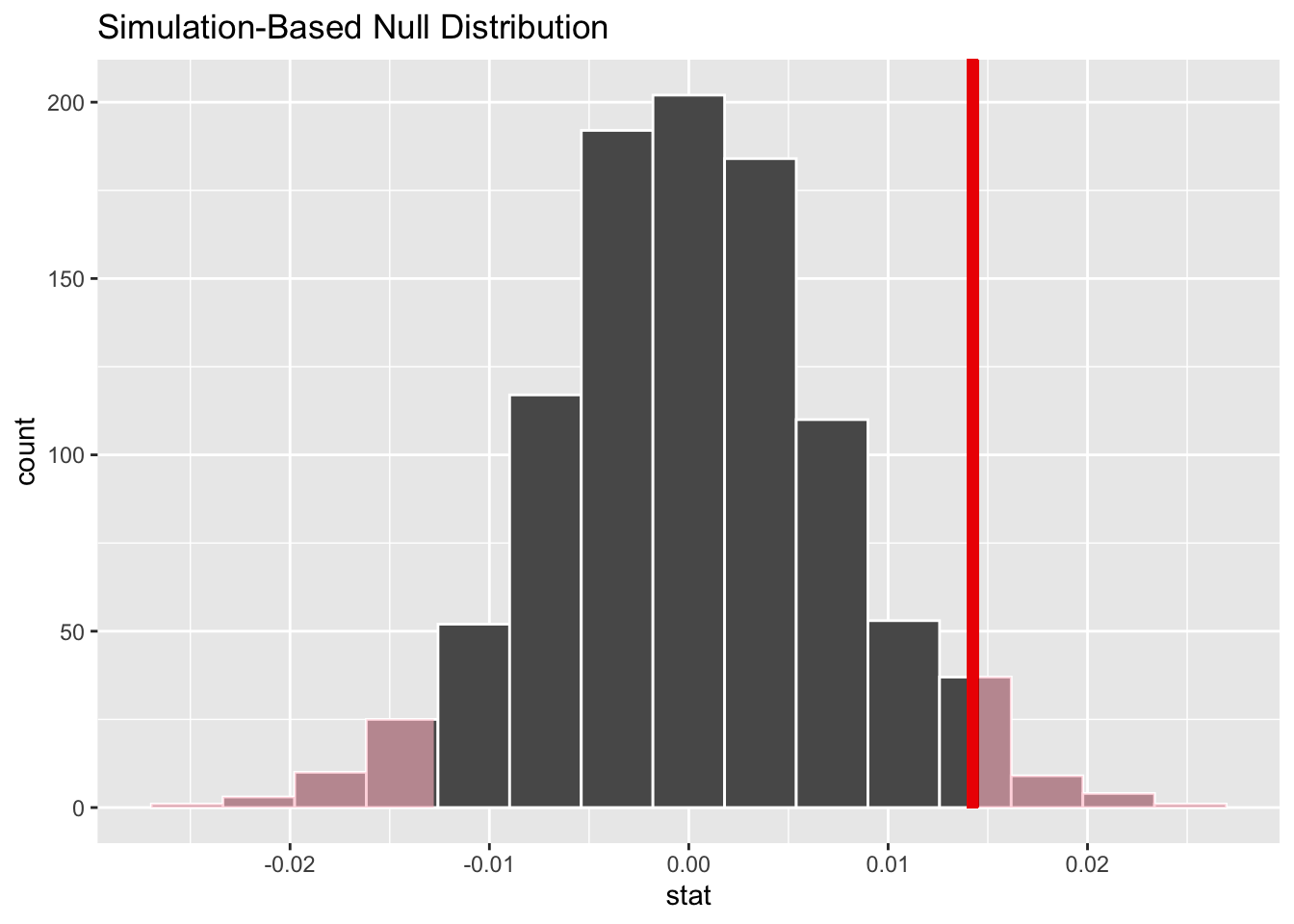

# geom_vline(xintercept = 0.0142428, color="red")
# The visualize function is from infer and it uses ggplot2 (see previous labs)

Comment on the histogram above. Did you expect it be centered about 0? Why or why not? Based on the location of the observed statistic, do you expect the p-value to be small or big?

Getting the P-value

In order to make a conclusion about the hypothesis test, we need to obtain the P-value. Recall that the P-value is the percent of observations at or above the observed statistic. It is a measure of the probability of getting a slope of 0.0142428 by chance alone assuming that the null hypothesis is true. The infer function for getting the P-value is get-p-value. See below:

simulated_slopes%>%
get_p_value(obs_stat = 0.0142428, direction="both")

# A tibble: 1 × 1
  p_value
    <dbl>
1   0.072

The Conclusion

Based on the p-value you found, write the conclusion for you hypothesis test in context.

Confidence Interval

We now want to create a bootstrap confidence interval to estimate the range within which expect to find the true population slope for the model predicting babies’ birth weight based on mothers’ age. To do this, we first create 1000 bootstrap samples using the code below. Take not of the difference between the code below and the one used earlier to generate the 1000 slopes for hypothesis test.

Bootstrap_samples <- births14 %>%
   specify (weight ~ mage) %>% 
   generate (reps = 1000, type = "bootstrap") %>%
   calculate (stat = "slope")

Once you run the above code, the object Bootstrap_samples will appear in the environment area. Click to view it. If we create a histogram to visualize the distribution of these values, what would you expect the histogram to look like?

Visualize The Bootstrap Distribution

We want to create a histogram to visualize the bootstrap distribution. We will also indicate the location of the observed statistic using a vertical red line.

visualize(Bootstrap_samples)+
  geom_vline(xintercept = 0.0142428, color="red")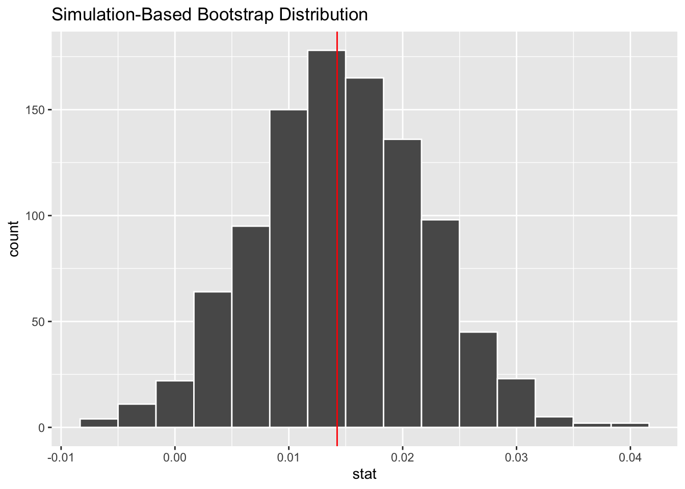

Getting the CI

To obtain the 95% confidence interval, we want to find the values (upper and lower) that incorporate the middle 95% of the data. Use teh code below:

Bootstrap_samples %>% get_ci(type = "percentile")

# A tibble: 1 × 2
   lower_ci upper_ci
      <dbl>    <dbl>
1 -0.000122   0.0292

#By default, get-ci returns the 95% CI unless you specify otherwise.

Interpreting the Confidence Interval

Write an interpretation for the confidence interval created above. Explain whether the results of the hypothesis test and interval agree?

Categorical Predictor Variable

In the example above, our predictor variable (age) and the response variable (weight) were numerical. If the predictor variable was categorical (2 levels), the test would be equivalent to testing the difference in means between the levels of the predictor variable. This test is popularly known as independent t-test. Let us make this more concrete:

Suppose want to answer the following research question: Do smoking mothers give birth to lighter babies than non-smoking mothers?

Hypotheses

There is no difference in weight between babies born to smoking mothers and those born to non smoking mothers.

\(H_0:\mu_1=\mu_2\) where, \(\mu_1\)= average weight of babies born to non-smoking mothers and \(\mu_2\)= average weight of babies born to smoking mothers.

Observed Statistic

The observed statistic is the difference in mean weight between babies born to smoking mothers and those born to non-smoking mothers in the data. To see the means side-by-side we can run teh code below:

births14 %>% 
 drop_na(habit, weight)%>%
 group_by (habit) %>%
 summarize(mean(weight))

# A tibble: 2 × 2
  habit     `mean(weight)`
  <chr>              <dbl>
1 nonsmoker           7.27
2 smoker              6.68

Thus, our observed statistic would be 0.59268.

Repeated Simulations

We can now run repeated simulations of to obtain more statistics to give us a null distribution. Take a moment to examine the code line by line. Most parts of the code should be familiar from previous labs.

set.seed(1234)
simulated_data_2 <-births14 %>% 
drop_na (habit, weight)%>%
     specify (weight ~ habit) %>%
     hypothesize (null ="independence") %>%
     generate (reps =1000, type ="permute") %>%
     calculate (stat ="diff in means", order =c("smoker", "nonsmoker"))

Visualize the Distribution

We can visualize the distribution and also include the observed statistic as before:

visualize(simulated_data_2) +  
  shade_p_value(obs_stat = 0.59268, direction ="two-sided")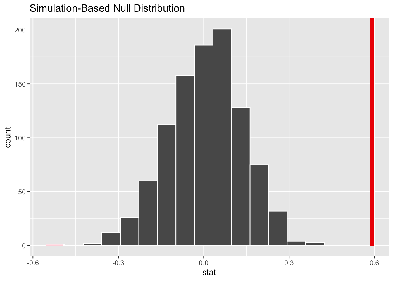

Based on the above histogram, what do you expect the P-value to be?

Get the P-value

Run the code below to get the P-value then write the conclusion in context.

simulated_data_2 %>%
  get_p_value (obs_stat = 0.59268, direction = "greater")

# A tibble: 1 × 1
  p_value
    <dbl>
1       0

Be sure to write the conclusion of your hypotheses in the context of the scenario.

Exercises

1. Rerun the hypothesis test for categorical predictor variable using slope as the statistic instead of diff in means. Compare your results with the ones done using the difference in means.

2. Create a confidence interval to estimate the parameter for exercise 1 above. Interpret the interval in context and explain whether it agrees with the test.