Code
data(duke_forest)More often than not, we are interested in specific variables or observations in a given larger data set. The question is, how do you pull a few cases or variables from a larger data set using R? At other times, you may want to modify a given variable for further analysis (e.g., in the duke_forest data set, you may want to divide the price by 1000 so you report in thousands). How do you do this? In this lab, you will learn about various techniques you can use to modify a data set to meet your preferences. Specifically, you will learn about the following functions:
To create your quarto file, follow the following steps:
Go to File>New File > Quarto document. In the title field use Introduction to Data Wrangling then write your name under the Author field. Change the output option to pdf.
Next, save the document as Lab_04. If you did it correctly, the file Lab_04.qmd should appear under the environment.
For more details on creating a quarto file, please check out lab_03a.
Once you create your new file, it comes with some default text and chunks. Feel free to reuse these (recommended option) or delete and start on a blank page. When reusing the template, be sure to rename headings accordingly and change the paragraphs to something more appropriate.
We will need the following packages in this lab. Load them in the first code chunk.
You can copy the following code for loading the packages:
library(openintro)
library(tidyverse)We will stick with the duke_forest data set. Please load the data set using the code below:
data(duke_forest)If you cannot see the data under the environment area, it is probably because you have not run the chunk containing the packages above. If you have the data set showing up, you can run ?duke_forest to access the documentation to learn more about this data if you need to but we have used this data set before.
Before you go too far, render the document to check if it is working correctly. Note that although you had loaded the data in a previous labs, you loaded it in different quarto documents. You have to load the data in every new quarto document that you create, otherwise, the document will not render.
The process of readying your data using various tools and functions before you run your analyses is often referred to as data wrangling. Some of these functions were listed above (select, mutate, etc). Let us explore each one of them:
We can now start with the main goal of this lab. First, the duke_forest data set has 13 variables. Suppose we are interested in just two of them - say cooling and price. We can use the select function to create a new data set from duke_forest that has the two variables that we need. Let us call this new data set duke_forest_a (you can use any name). See the code below:
duke_forest_a <- duke_forest |>
  select (cooling, price)
When you run the above code, a new object (duke_forest_a) will pop up in the environment area. Click on this object to see it.
Suppose we want to divide the price by 1000 so that we report the process in thousands instead of the huge numbers that we saw in previous labs. To do this, we use the mutate function on the the duke_forest_a data set (you can also use the original data set). Study the code below then copy and paste to run it:
duke_forest_b <- duke_forest_a |>
  mutate(new_price = price/1000)
This code creates a new variable and now we have three variables instead of two. We have assigned the name new_price to the new variable. Note also that the new data set is given a new name duke_forest_b. For beginners, it is a good idea to use different names so you keep track of what you are doing at every step.
Another common scenario that arises is when you want to split a given numerical variable into some categories. For example, suppose you want to designate the house prices as high cost or low cost based on price. Let us say you consider houses over $ 450,000 to be high cost and those less than $ 450,000 to be low cost. You can do this using the mutate function and the ifelse function as shown below:
duke_forest_price <- duke_forest |>
mutate("cost" =ifelse(price>450000, "High_Cost", "Low_Cost"))
With this new data, you can create a simple bar plot to visualize the distribution of houses by cost as shown below:
ggplot(data=duke_forest_price, aes(x=cost, fill=cost))+
  geom_bar()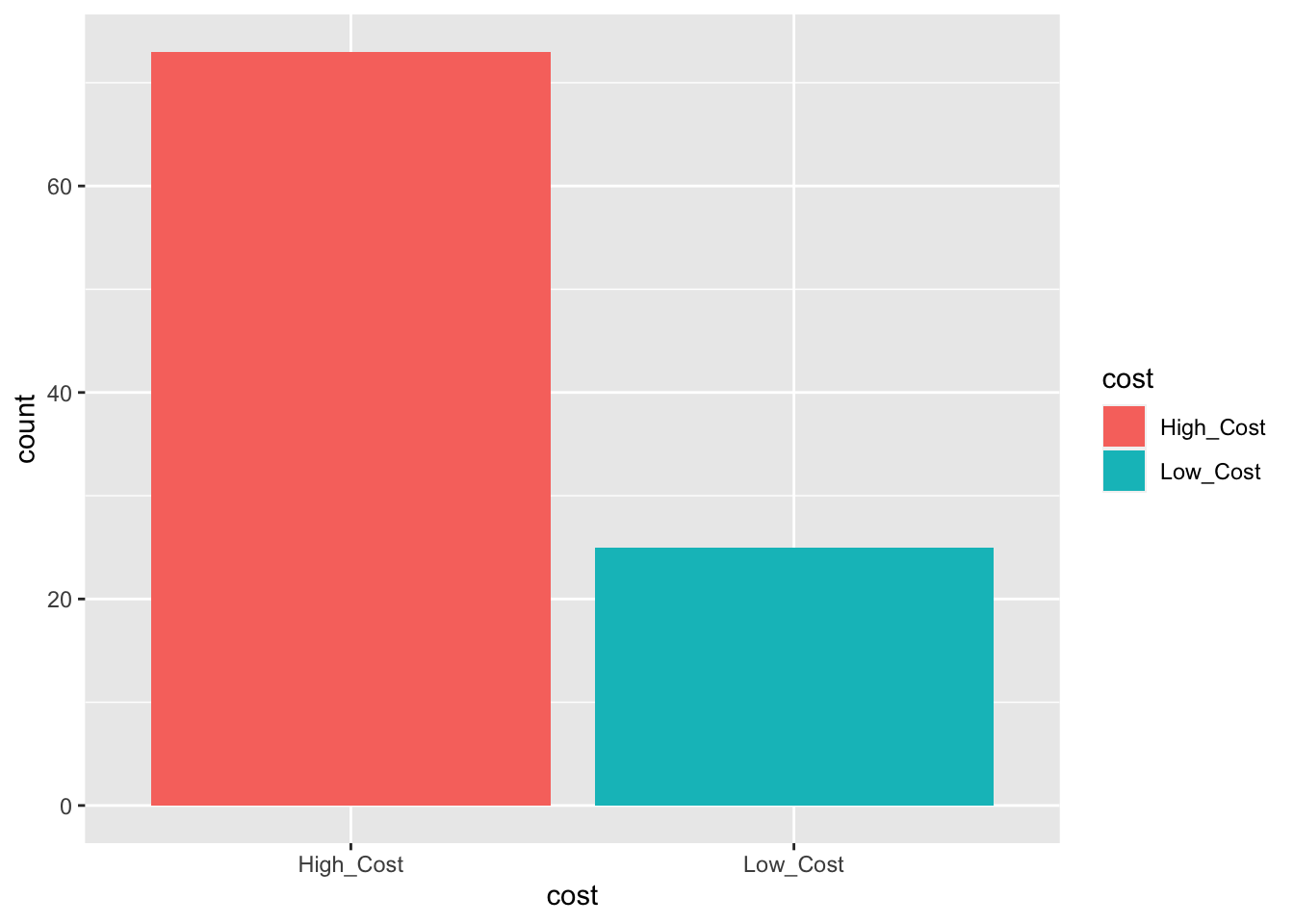
If you wanted to have average price on the y-axis, you can add the summary and fun arguments in the geom_bar as shown below:
ggplot(data=duke_forest_price, aes(x=cost, y = price, fill=cost))+
  geom_bar(stat = "summary", fun="mean")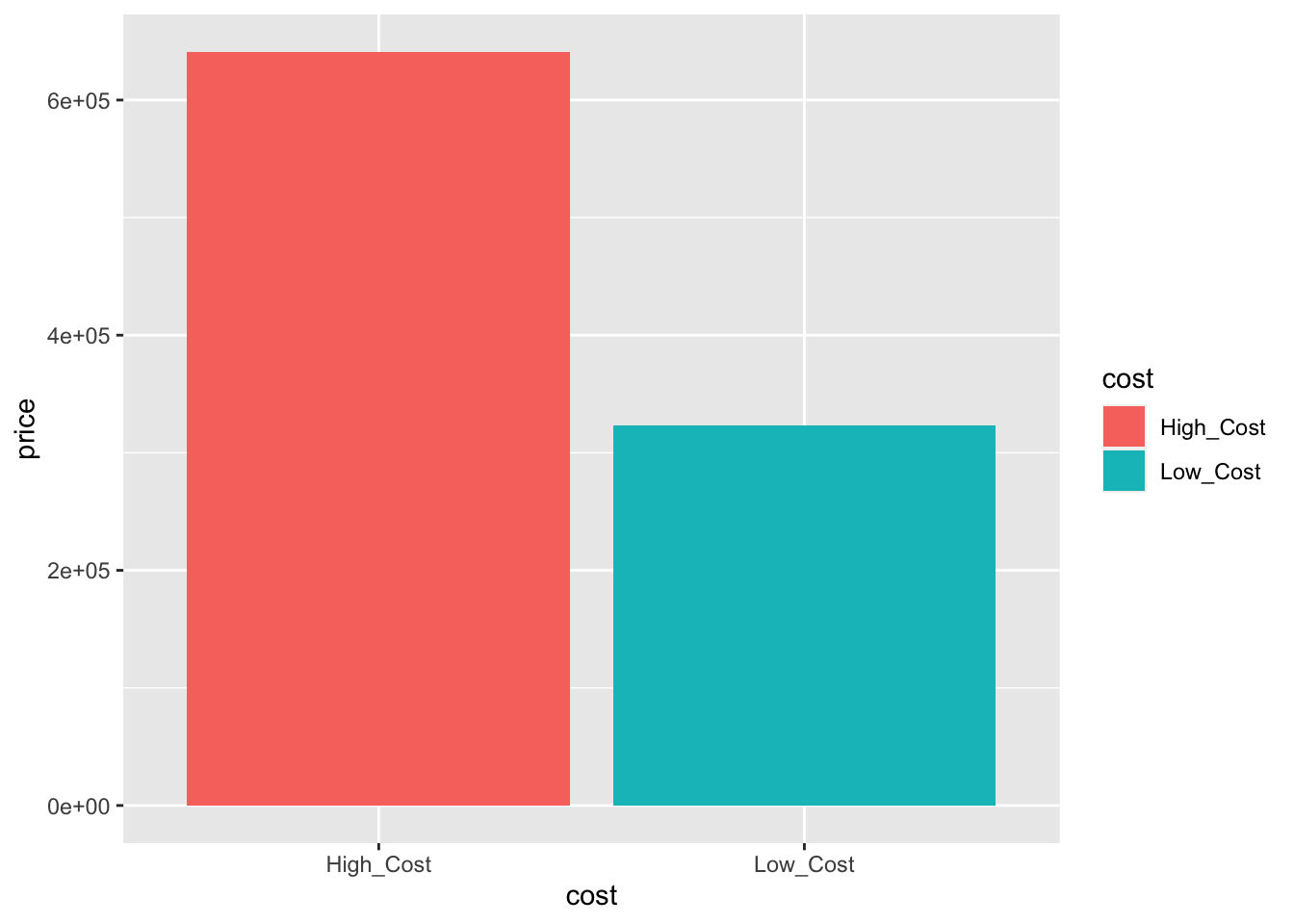
# Notice that price is in thousandsSuppose we want to create a new data set that has houses with central cooling only. Note that cooling is a variable and we are interested in one of its levels only (i.e., central). To do this, we can use the filter function as shown below:
duke_forest_c <- duke_forest_b |>
filter (cooling == "central")
#Comment: Note the use of double == signs, not just =
When you run the above code, you get a new data set named duke_forest_c that has only 45 cases, meaning only 45 houses had central cooling. You can click on the data set to inspect it.
You can also filter by a numerical variable. For example, you may want to isolate houses for which price is under \(\$250,000\). e use the filter function as follows:
duke_forest_d <- duke_forest |>
filter(price<250000)
Question:
You can also filter by multiple criteria. For example, to isolate houses that cost less than 250,000 AND that have central cooling, we can use the filter function as shown below:
duke_forest_e <- duke_forest |>
filter(price<250000, cooling=="central")
Challenge Question:
If you see any cells (variable values) with NA, it means that value is missing for some reason. For example, the respondent may not have answered that question or the person entering the data skipped that value by mistake.
Some analyses may not work properly with NA values included. In the duke_forest data set, there are several NA values in the variable hoa (whether house belongs to Home Owners Association). We can drop these as follows
duke_forest_f<- duke_forest|>
  drop_na(hoa)
In the above code, we use the drop_na function and then specify the variable from which we want to drop the NA values. You can have several variables here as long as you separate them using commas.
Group_by is a special kind of filtering that is commonly used alongside a summarize function. Suppose you want to answer the question; Are houses with central cooling pricier on average than those without central cooling?.
Here, you first use the group_by function to group the cases by cooling, then run the summarize function and call the mean. Study the code below and try it for yourself:
duke_forest |>
  group_by (cooling) %>%
  summarize(mean(price))
# A tibble: 2 × 2
cooling `mean(price)`
<fct> <dbl>
1 other 516776.
2 central 610688.Question:
price by cooling for houses in the duke_forest data set.(2 pts) Load the data set called loan50 into your work space.
(4 pts) Use the select function to extract the variables homeownership, annual_income, and loan_purpose from the loan50 data set and store the new data set as loan50a.
(4 pts) Use the mutate function to create a new data set (store it as loan50b) from the loan50a data set. In this new data set, annual_income should be in thousands (i.e., divided by 1000).
(4 pts) Use the filter function to create a new data set (store it as loan50c) from the loan50b data set created above. In this new data set, annual_income should be greater than 50000. How mnay people make over 50000?
(6 pts) Do people who own their homes make more on average than people who do not own their homes? To answer this question, use the group_by and summarize functions.